Using USim to Solve Multi-Species Reactive Flows
Multi-species transport in cylindrical coordinates along with reactions is demonstrated in this example. A hypothetical gas consisting of three species N2,N,O2 is considered here. Mass transport of individual species is solved along with Euler equations. Rate equations are solved in USim to obtain the change in concentration of the species due to chemical reactions. The rate of change of species is obtained using reaction rates and then added to the species transport as sources. Similarly the the change in energy is incorporated using energy of formation of each of the species. The related input file can be found in Blunt-Body Reentry Vehicle (ramC.pre) example of USimHS.
Contents
Multi-Species Mass Transport
Species mass transport fluxes are evaluated using the classicMuscl updater and Eigenvalues values of the Euler equation (see Using USim to solve the Euler Equations). The updater block is as given below.
<Updater hyperSpecies>
  kind = classicMuscl2d
  timeIntegrationScheme = none
  numericalFlux = localLaxFlux
  limiter = [minmod, minmod, minmod, none]
        variableForm = conservative
  cfl = CFL
  onGrid = domain
  in = [speciesDens, q, p, a]
  out = [speciesDensNew]
  equations = [speciesContinuity]
  sources = [multiSpeciesAxiSrc]

  <Equation speciesContinuity>
    useParentEigenvalues = true
    inputVariables = [speciesDens, q]
    kind = multiSpeciesSingleVelocityEqn
    numberOfSpecies = NSPECIES

    <Equation euler>
      kind = realGasEosEqn
      inputVariables = [q, p, a]
      numSpecies = NSPECIES
    </Equation>

  </Equation>

  <Source multiSpeciesAxiSrc>
     kind = multiSpeciesSym
     symmetryType = cylindrical
     numberOfSpecies = NSPECIES
  </Source>
</Updater>
This block uses Equation sub-block and a Source block. The mass fluxes are computed in the Equation block using the Eigenvalues of conservative variables q. Here q contains the conservative variables of realGasEosEqn equation. The equation of state is user specified, hence it requires pressure p and speed of sound a as inputs. The Source block computes the sources due to additional terms in cylindrical coordinates. The fluxes evaluated in both of the sub-blocks are added to the out variable speciesDensNew.
Mass Diffusion
Mass diffusion source for the multi-species can computed using the following block. This block uses diffusion (1d, 2d, 3d) operator to compute the diffusion source, with the derivative specified as diffusion, numScalars is the number of species, isRadial is true for cylindrical coordinates, and the input variables are species density and diffusion coefficient D. out variable diffSrc contains the output.
<Updater computeDiffSrc>
  kind = diffusion2d
  onGrid = domain
  derivative = diffusion
  numScalars = NSPECIES
  coefficient = 1.0
  numberOfInterpolationPoints = 8
  isRadial = true
  in = [speciesDens,D]
  out = [diffSrc]

</Updater>
Rate of Change of Density
The following equation block shows the computation of rate of change of density three species due to two reactions. In order to use this block, a nodalArray variable consisting of the species densities speciesDens has to be initialized, another array to add the density change rates speciesDensNew should be declared, and an nodalArray with average temperature of the species. The two reactions are N2 + N2 -> N + N + N2 and N2 + O2 -> N + N + O2. The equation block follow.
<Updater sourceUpdater>
  kind = equation2d
  onGrid = domain

  in = [speciesDens, temperature]
  out = [speciesDensNew]

  equations = [reactionSrc]

   <Equation reactionSrc>
     kind = reactionTableRhs
     outputEnergyRate = 0
     maxRate = 1.0e28
     species = [N2, N, O2]
     fileName = airReaction.txt
   </Equation>
</Updater>
The attributes used in the above block are
| option: | kind (string) Specifies the type of updater. Here it is equation2d |
|---|---|
| option: | in (nodalArray) Names of the required nodalArray inputs. In this example, those are speciesDens, temperature |
| option: | out Name of the output variable. |
| option: | equations (string) Name of the equation. Here the name is reactionSrc |
Attributes within the Equation sub blocks
| option: | kind (string) Type of equation. In this example, it is reactionTableRhs |
|---|---|
| option: | outputEnergyRate (boolean) option to compute reaction energy. it is chosen to be false in this demo. |
| option: | maxRate (real number) An option to introduce artificial limit on the maximum value of reaction rate. It is useful in stabilizing the solution at reasonably small time steps. |
| option: | species (list of strings) Names of the species considered. |
| option: | fileName (string) Name of the Multi-Species Data Files. |
Within the Equation Any number of reactions can be included by simply adding those to Multi-Species Data Files.
Chemical Energy
The energy of formation is computed using the following Updater block. The total energy of formation of all the species is added to get the mixture’s energy. This energyOfFormation is added to internal energy in the energy equation. Hence during the initialization, the initial value of energyOfFormation should be computed using the initial densities of species and added to the energy density variable.
<Updater computeChemEn>
  kind = equation2d
  onGrid = domain

  in = [speciesDens,cpR,temperature]
  out = [chemEn]

  <Equation cp>
    kind = transportCoeffSrc
    coeff = chemicalEnergy
    numSpecies = NSPECIES
    fileName = airReaction.txt
  </Equation>
</Updater>
The attributes used in the above block are
| option: | kind (string) Specifies the type of updater. Here it is equation2d |
|---|---|
| option: | in (nodalArray) Names of the required nodalArray inputs. In this example, those are speciesDens, cpR, temperature. specisDens is the number densities of all species, cpR is specific heats. temperature is average temperature of species. speciesDens and cpR are arrays with size equal to the number of species. |
| option: | out Name of the output variable. contains the energy of formation. This variable will have only one component. |
Addition of sources in time integrator
Two updaters are here, one for integrating the conservative variables q and species density speciesDens. The other is to integrate time rate of change of species due to reactions in using detailed explanation of the attributes is found in multiUpdater (1d, 2d, 3d).
<Updater rkUpdaterFluid>
  kind = multiUpdater2d
  onGrid = domain

  in = [q,speciesDens]
  out = [qnew,speciesDensNew]

  <TimeIntegrator rkIntegrator>
    kind = TIMEINTEGRATION_METHOD
    ongrid = domain
    scheme = TIMEINTEGRATION_SCHEME
  </TimeIntegrator>

  <UpdateSequence sequence>
    loop = [boundaries,hyper]
  </UpdateSequence>

  <UpdateStep boundaries>
     updaters = [bcOutflowSpecies, bcInflowSpecies, bcAbWallSpecies1, bcAbWallSpecies2, bcAbWallSpecies3, computeChemEn, computeTemperature, temperatureCorrector, bcFluidTempAxis, bcFluidTempWall, bcFluidTempInflow, bcFluidTempCopy, bcSurfTemp, bcOutflow, bcInflow, bcAxis, bcAbWall1, bcAbWall2, bcAbWall3]
     syncVars = [speciesDens,chemEn, temperature, surfTemp, q]
  </UpdateStep>

 <UpdateStep hyper>
 operation = "integrate"
  updaters = [computeChemEn, computeTemperature, temperatureCorrector, computeCpAvg, computeMwAvg, computeGammaAvg, computeViscosity, computeThermalCoefficient, computeGasPressure, computeElectronPressure, computeHvpPressure, bcPressureWall1, bcPressureWall2, bcPressureWall3, computeSoundSpeed, computeKinematicViscosity, computeThermalDiffusivityFluid, computeVelocity,computeViscousSource,hyper, hyperSpecies, addViscousSource]
  syncVars = [temperature, p,a,velocity,viscousSource,qnew,speciesDensNew]
</UpdateStep>
Boundary conditions are applied on species using bcOutflowSpecies, bcInflowSpecies, bcAbWallSpecies1, bcAbWallSpecies2, bcAbWallSpecies3. Energy of formation and temperature are computed using computeChemEn, computeTemperature. Remember that, energy of formation is required to compute temperature. Boundary conditions on temperature are then applied using bcFluidTempAxis, bcFluidTempWall, bcFluidTempInflow, bcFluidTempCopy, bcSurfTemp updaters. Finally boundary conditions are applied to bcOutflow, bcInflow, bcAxis, bcAbWall1, bcAbWall2, bcAbWall3 conservative variables.
Energy of formation, computeChemEn is evaluated and then temperature is computed using the updater computeTemperature. The properties are evaluated using computeCpAvg for average value of constant pressure specific heat of species, computeMwAvg for the average molecular weight, and computeGammaAvg for average gamma of the mixture. Viscosity an thermal conductivity are evaluated using computeViscosity, computeThermalCoefficient. The total pressure of the gas, electron pressure and heavy particle pressure are computed using computeGasPressure, computeElectronPressure, computeHvpPressure updaters respectively. The pressure is copied into the ghost layers using the boundary condition updaters bcPressureWall1, bcPressureWall2, bcPressureWall3. Pressure boundary condition is applied for realGasEosEqn. Then computeSoundSpeed is evaluated. computeKinematicViscosity, computeThermalDiffusivityFluid are evaluated to obtain kinematic viscosity and thermal diffusivity. These are required for time step restriction based on diffusion. Velocity of fluid is evaluated using computeVelocity and then viscous source is computed computeViscousSource. Convective fluxes of conservative variable are computed in ‘hyper’ and stored in qnew. Convective fluxes of species are stored in speciesDensNew. Viscous source is added to qnew using addViscousSource.
The change in density due to reactions is added to species density and integrated in the following Updater. The updater sourceUpdater evaluates and adds the rate of change of density to the species equations. The resulting equations are integrated using localOdeIntegrator (1d, 2d, 3d) method.
<Updater sourceUpdater>
    kind = localOdeIntegrator2d

    onGrid = domain

    in = [speciesDens, temperature]

    out = [speciesDensNew]
    integrationScheme = bulirschStoer
    relativeErrorTolerance = 1.0e9
    equations = [reactionSrc]
     <Equation reactionSrc>
       kind = reactionTableRhs
       outputEnergyRate = 0
       maxRate = MAXRATE
       species = [N2, N, O2, O, NO, NO_p1, e, Ca, Na, K]
       fileName = airReaction.txt
    </Equation>

  </Updater>
An Example Simulation
The Blunt body reentry example of the USimHS demonstrates each of the concepts described above using 7 species model of air. The considered 7 species are \(N2, N, O2, O, NO, NO+, e\). Executing the Blunt body reentry input file within USimComposer and switching to the Visualize tab yields the plot shown in Fig. 8.
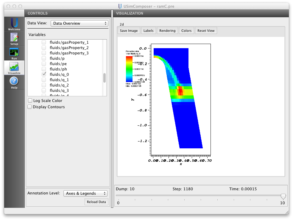
Figure 8: Visualization tab in USimComposer after executing the input file for the tutorial.