Radio Communication Blackout (ramCEM.pre)
Keywords:
-
hypersonic, reentry, plane-wave, blackout
Problem description
This example simulates the propagation of electro-magnetic wave through plasma. The objective is to simulate the communication blackout on re-entry vehicles. A plane sine wave is sent from the left hand side face of the domain. Maxwell’s equations are then solved to get the electric and magnetic field components in the simulation domain.
This simulation requires both a USimHS and USIMHEDP license.
Creating the run space
The Radio Communication Blackout example is accessed from within USimComposer by the following actions:
- Select the New from Template menu item in the File menu.
- In the resulting New from Template window, expand USimHS or USimHEDP.
- Select Radio Communication Blackout and press the Choose button.
- In the resulting dialog, press the Save button to create a copy of this example in your run area.
The basic variables of this problem should now be settable in text boxes in the right pane of the “Setup” window.
Input file features
The following parameters can be varied:
- TEND - Simulation end time (seconds)
- EM_FREQUENCY - wave frequency
- EM_CYCLES - number of EM wave cycles to evolve for
- NUMDUMPS - Number of data dumps during the simulation
- GENERATE_INITIAL_CONDITION - Generate the evolved plasma distribution on the mesh
- GRIDFILE - name of grid file
- REACTIONS_ATOMIC_DATA - name of the consisting of reactions and atomic data
- SPEED - free stream velocity
- AOA - angle of attack
- FREESTREAM_DENSITY - free stream density
- FREESTREAM_TEMPERATURE - free stream temperature
- SURFACE_EMISSIVITY - emissivity of the surface
- GAS_EMISSIVITY - emissivity of the hot gas in the vicinity of surface
- MW1_1 - molecular weight of species 1
- ABP01_1 - reference pressure of species 1
- ABDH1_1 - evaporation enthalpy of species 1
- ABT01_1 - reference temperature of species 1
- CFL_CONVECTIVE - CFL condition number for convective terms
- VISCOUS_DIFF_TIMESTEP_FACTOR - Factor to further decrease the internally computed time step based on kinematic viscosity
- THERMAL_DIFF_TIMESTEP_FACTOR - Factor to further decrease the internally computed time step based on thermal diffusicity
- BASEMENT_TEMPERATURE - least possible temperature in the domain (K)
Note that the input file comes with an externally generated unstructured mesh using cubit.
Running the simulation
This example simulates the propagation of an EM wave through the plasma layer surrounding the re-entry vehicle. The first step in the simulation is to generate this plasma distribution, accomplished by setting GENERATE_INITIAL_CONDITION = True (the default). With this choice, generate the plasma distribution by proceeding as follows:
- Press the Save And Process Setup button in the upper right corner.
- Proceed to the run window as instructed by pressing the Run button in the left column of buttons.
- To run the file, click on the Run button in the upper right corner. of the window. You will see the output of the run in the right pane. The run has completed when you see the output, “Engine completed successfully.”
Once the simulation has completed, return to the “Setup” window and set GENERATE_INITIAL_CONDITION = False and increase the NUMDUMPS to 20. Then:
- Press the Save And Process Setup button in the upper right corner.
- Proceed to the run window as instructed by pressing the Run button in the left column of buttons.
- Chose the restart dump number equal to the final dump file from the previous run.
- To run the file, click on the Run button in the upper right corner. of the window. You will see the output of the run in the right pane. The run has completed when you see the output, “Engine completed successfully.”
Visualizing the results
After performing the above actions, continue as follows:
- Proceed to the Visualize window as instructed by pressing the Visualize icon in the workflow panel.
- Press the Open button to begin visualizing.
- Expand Scalar Data and click the check box for fluids/em_1 to visualize the y-component of electric field as shown in Figure 74. Refer to maxwellEqn to see the definitions of remaining components.
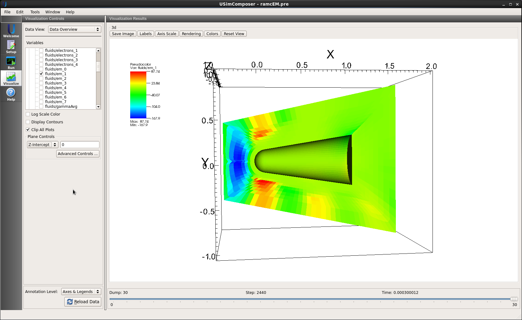
Figure 74: Plane EM wave propagation through plasma layer on RAMC during re-entry.
Further experiments
- Change the wave frequency.
- Run the simulation without plasma. Do not use the restart option and make TEND = 0 and GENERATE_INITIAL_CONDITION = False.
- Parallel: carry out the simulation on 2 and 8 cores using the MPI option.