Anisotropic Poisson (anisotropicPoisson.pre)¶

Problem description¶

This example demonstrates the anisotropic Poisson solve that can be used for the electric potential, heat transfer, magnetic field diffusion, and wherever a Poisson’s equation has to be solved. A source varying in space and time is considered. The source has a sine wave variation at a frequency of 1 MHz. The coefficients are assumed to be different in x,y, and z directions. Source is given by s = (6x+12y+18z)*sin(wt). Simulation is performed for a duration of one cycle. For CX=1, CY=2, and CZ=3, the result would be x^3+y^3+z^3.

This simulation can be performed with a USimHEDP license.

Creating the run space¶

The Anisotropic Poisson example is accessed from within USimComposer by the following actions:

• Select the New from Template menu item in the File menu.
• In the resulting New from Template dialog, expand USimBase: Basic Physics Capabilities.
• Select Anisotropic Poisson and press the Choose button.
• In the Choose a name for the new runspace dialog, press the Save button to create a copy of this example in your run area.
• Press the Save And Process Setup button in the upper right corner of the Editor pane.

The basic example variables are editable in the Editor pane of the Setup window. After any change is made, the Save and Process Setup button must be pressed again before a new run commences.

Input file features¶

Primary variables are:

• FREQUENCY - source variation frequency
• CX, CY, CZ - coefficients in the x,y,z directions
• NX, NY, NZ - Number of cells in the x,y,z directions
• NUMDUMPS - Number of data dumps during the simulation

Running the simulation¶

After performing the above actions, continue as follows:

• Proceed to the Run window as instructed by pressing the Run icon in the workflow panel.
• To run the simulation, click on the Run button in the upper right corner of the Logs and Output Files pane.

You will also see the engine log output in the Logs and Output Files pane. The run has completed when you see the output, “Engine completed successfully.”

Visualizing the results¶

After performing the above actions, continue as follows:

• Proceed to the Visualize window as instructed by pressing the Visualize icon in the workflow panel.
• Press the Open button to begin visualizing. The left pane has all of the output variable from the simulation. Expand the ‘Scalar Data’ field to see ‘fluids/coeff_0..._9’ (tensor of the diffusion coefficients), phi (scalar potential), and rho (source on the right hand side of the Poisson’s equation).
• Select the variable ‘phi’ and drag the slider at the bottom of the Visualization Results pane to the right to see potential at the positive peak of the source simulation. Check the ‘Display Contour’ option and hold+move the cursor along the contours to set an orientation as shown in Fig. 83.

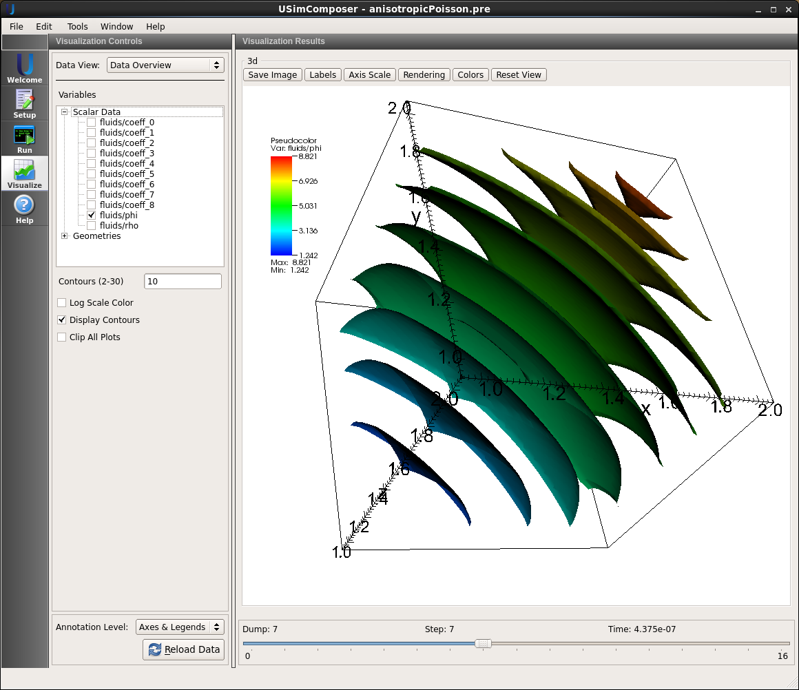
Figure 83: Visualization of the time varying scalar potential

Further experiments¶

• Change the resolution of the grid by setting NX, NY, NZ to 64 or 128 to see more refined results.