Merging Plasma Jets (plasmaJetMerging.pre)¶

Problem description¶

This problems shows plasma jet merging as investigated for the Los Alamos Plasma Liner Experiment by HyperV technologies. An ideal MHD model with general equation of state and bremsstrahlung radiation is used along with the plasma jet updater. By modifying the input file an arbitrary number of plasma jets can be included at arbitrary angles with respect to each other.

Creating the run space¶

The Merging Plasma Jets example is accessed from within USimComposer by the following actions:

• Select the New from Template menu item in the File menu.
• In the resulting New from Template dialog, expand USimHEDP: High Energy Density Plasmas.
• Select Merging Plasma Jets and press the Choose button.
• In the Choose a name for the new runspace dialog, press the Save button to create a copy of this example in your run area.
• Press the Save And Process Setup button in the upper right corner of the Editor pane.

The basic example variables are editable in the Editor pane of the Setup window as shown below. After any change is made, the Save and Process Setup button must be pressed again before a new run may commence.

Input file features¶

The following parameters can be modified to look at the effect on plasma jet merging:

• DIM - Dimension of the simulation (2 or 3)
• T_EV - Plasma temperature in electron volts
• N0 - Peak jet density in number per meter cubed
• AR - Ion species atomic mass
• U - Jet velocity towards the origin
• B0 - Uniform initial magnetic field in the Z direction
• BX - Uniform initial magnetic field in the X direction
• GAMMA - Specific heat ratio of plasma
• JET_INIT_LENGTH - Length of the region to initialize the jet.
• JET_INIT_WIDTH - Width of the region to initialize the jet.
• JET_DENSITY_FUNCTION - Function that hape of the jet as a function of parallel (x) and perpendicular (r) directions
• RAD - Distance from the origin of the start of each plasma jet
• CFL - CFL condition for the simulation
• TEND - Simulation end time (seconds).
• NUMDUMPS - Number of data dumps during the simulation
• PRESSURE_FACTOR - Vacuum pressure factor which is the ratio of background pressure to peak initial pressure
• DENSITY_FACTOR - Vacuum density factor which is the ratio of background density to peak initial density
• CORRECTION_SPEED - Magnetic field divergence correction speed. Should be on the order of the fastest MHD wave speed in the simulation.
• NUMERICAL_FLUX - specifies the Riemann solver used to calculate an upwind approximation to the flux tensor. For hydrodynamic problems, options include localLaxFlux, hlleFlux, hllcEulerFlux. For magnetohydrodynamic problems, options include localLaxFlux, hlleFlux, hlldMhdFlux, fWaveFlux. For more general systems, options include localLaxFlux, hlleFlux, fWaveFlux.
• TIME_ORDER - first,second,third,fourth sets the order of accuracy for the time-integration.
• LIMITER - muscl,minmod,none specifices the spatial limiting method used in reconstructing primary variables to use to ensure that method remains total value diminishing (TVD).
• NX - Number of cells in the x direction
• NY - Number of cells in the y direction
• NZ - Number of cells in the z direction (3D only)
• X_MIN - lower X position of grid
• X_MAX - upper X position of grid
• Y_MIN - lower Y position of grid
• Y_MAX - upper Y position of grid
• Z_MIN - lower Z position of grid (only in 3D)
• Z_MAX - upper Z position of grid (only in 3D)

Running the simulation¶

After performing the above actions, continue as follows:

• Proceed to the Run window as instructed by pressing the Run icon in the workflow panel.
• To run the simulation, click on the Run button in the upper right corner of the Logs and Output Files pane.

You will also see the engine log output in the Logs and Output Files pane. The run has completed when you see the output, “Engine completed successfully.”

Visualizing the results¶

After performing the above actions, continue as follows:

• Proceed to the Visualize window as instructed by pressing the Visualize icon in the workflow panel.
• Press the Open button to begin visualizing.
• Expand Scalar Data and click the check box for fluids/density to visualize fluid densities.
• Drag the slider at the bottom of the Visualization Results pane to move through the simulation in time. The fluid density distribution is early on in the simulation is shown in Fig. 89.

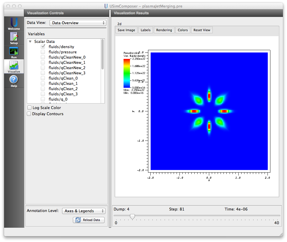
Figure 89: Visualization of density in Merging Plasma Jets Merging example

Further experiments¶

• The default simulation has the background magnetic field set to 0. Set the background magnetic field B0=0.01 and run the simulation again. By visualizing \(q_{7}\) in the visualization window you will be able to see the compression of the Z magnetic field from the incoming jets.
• We typically run these simulations with a background density factor of about \(1\times 10^{-6}\) the initial peak density to simulate the vacuum. If this value is raised significantly by, for example, increasing DENSITY_FACTOR to \(1\times 10^{-1}\), you will see the jets plow into the background fluid, illustrating why it is important to maintain a low background density for these types of problems.