Turbulent Flow Over Flat Plate (flatPlate.pre)¶

Problem description¶

This problem demonstrates boundary layer formation for subsonic flow over a flat plate, based on the problem described at http://turbmodels.larc.nasa.gov/flatplate.html. Two choices of Reynolds-Averaged Navier Stokes turbulence models are available: the Chien kEpsilon model described at http://turbmodels.larc.nasa.gov/ke-chien.html and the kOmega SST model described at http://turbmodels.larc.nasa.gov/sst.html.

This simulation can be performed with a USimHS license.

Creating the run space¶

The Flat Plate example is accessed from within USimComposer by the following actions:

• Select the New from Template menu item in the File menu.
• In the resulting New from Template dialog, expand USimHS: Hypersonics.
• Select Flow over Flat Plate and press the Choose button.
• In the Choose a name for the new runspace dialog, press the Save button to create a copy of this example in your run area.
• Press the Save And Process Setup button in the upper right corner of the Editor pane.

The basic example variables are editable in the Editor pane of the Setup window. After any change is made, the Save and Process Setup button must be pressed again before a new run commences.

Input file features¶

The input file allows the user to set a variety of problem parameters related to the physics, initial conditions, domain and solver used for boundary layer formation for subsonic flow over a flat plate.

The following parameters control the simulation physics:

• USE_KEPSILON = True,False - selects whether to evolve the problem using the Chien kEpsilon model (USE_KEPSILON = True) or the kOmega SST model (USE_KEPSILON = False).
• MACH_NUM - sets the ratio of the flow velocity to the sound speed (the Mach number).
• T_ATM - sets the flow temperature in Kelvin.
• P_ATM - sets the flow pressure in Pascals.
• TURBULENT_INTENSITY - sets the intensity of turbulent fluctuations captured by RANS Model.
• TURBULENT_REYNOLDS_NUMBER - is a dimensionless parameter describing ratio of turbulent viscosity to characteristic length scale.
• GAS_GAMMA - sets the adiabatic index (ratio of specific heats) of the fluid.

The following parameters control the dimensionality, domain size and resolution of the simulation:

• VERTICAL_ZONES - sets the number of zones in the direction perpendicular to the flow.
• VERTICAL_SIZE - sets the size of the domain in the direction perpendicular to the flow.

The following parameters the length of the simulation and data output:

• TEND - sets the end time for the simulation.
• NUMDUMPS - sets the number of data dumps during the simulation
• WRITE_RESTART = False,True - tells USim to output data necessary to restart the simulation. If this parameter is set to False then the Restart at Dump Number functionality in the Standard tab under Runtime Options in the Run window will not be available.

The following parameters control the USim solvers used to evolve the problem:

• HYPERBOLIC_TIME_ORDER = first,second,third,fourth - sets the order of accuracy for the hyperbolic system time-integrator.
• DIFFUSION_TIME_ORDER = first,second - sets the order of accuracy for the diffusion system time-integrator.
• DEBUG = False,True - sets whether to output data for debugging a run. Warning: this will output A LOT of information!

Running the simulation¶

After performing the above actions, continue as follows:

• Proceed to the Run window as instructed by pressing the Run icon in the workflow panel.
• To run the simulation, click on the Run button in the upper right corner of the Logs and Output Files pane.

You will also see the engine log output in the Logs and Output Files pane. The run has completed when you see the output, “Engine completed successfully.”

Visualizing the results¶

After performing the above actions, continue as follows:

• Proceed to the Visualize window as instructed by pressing the Visualize button in the left column of buttons.
• Press the “Open” button to begin visualizing.
• To visualize the fluid density, expand the Scalar Data tab and click the check box for fluids/velocity.
• Drag the slider at the bottom of the visualization window to move through the simulation in time. The velocity distribution at the end of the simulation is shown in Fig. 93.

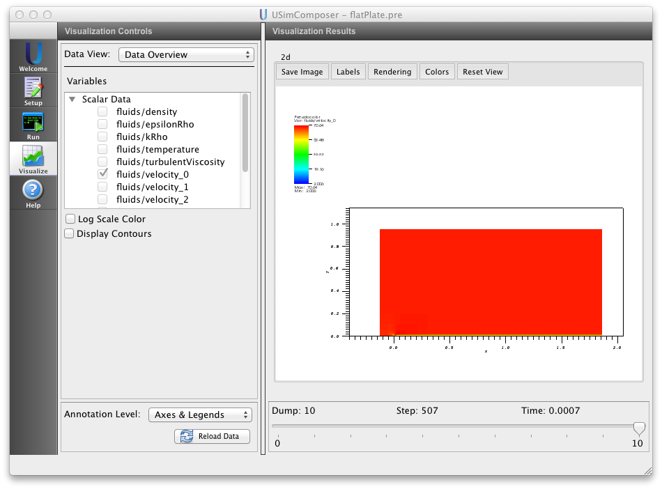
Figure 93: Visualization of the flow velocity flow over a flat plate as a color contour plot.

Further experiments¶

• Set USE_KEPSILON to False to use the KOmega SST RANS turbulence model.
• Increase VERTICAL_ZONES to study convergence of the boundary layer properties.