Flow over a Cylindrical Rod (highSpeedRod.pre)¶

Problem description¶

This problem demonstrates aerothermal heating of a cylindrical body moving at Mach 23. The air surrounding the shock regions dissociates and ionizes. This simulation considers 7 species air chemistry model and simulates the flow at sea level. Viscous and conductive terms appropriate for a Sutherland viscosity model are implemented and are accelerated using Super Time Stepping techniques.

This simulation can be performed with a USimHS license.

Creating the run space¶

The Flow over a Cylindrical Rod example is accessed from within USimComposer by the following actions:

• Select the New from Template menu item in the File menu.
• In the resulting New from Template dialog, expand USimHS: Hypersonics.
• Select Flow over a Cylindrical Rod and press the Choose button.
• In the Choose a name for the new runspace dialog, press the Save button to create a copy of this example in your run area.
• Press the Save And Process Setup button in the upper right corner of the Editor pane.

The basic example variables are editable in the Editor pane of the Setup window. After any change is made, the Save and Process Setup button must be pressed again before a new run commences.

Input file features¶

The input file allows the user to set problem parameters. They are:

• FREESTREAM_DENSITY - free stream density
• FREESTREAM_TEMPERATURE - free stream temperature
• MACH_NUM - flow mach number
• NUMDUMPS - number of data dumps during the simulation
• GRIDFILE - mesh file for the simulation

The default choices for the free stream density and temperature are appropriate for sea level.

Running the simulation¶

After performing the above actions, continue as follows:

• Proceed to the Run window as instructed by pressing the Run icon in the workflow panel.
• To run the simulation, click on the Run button in the upper right corner of the Logs and Output Files pane.

You will also see the engine log output in the Logs and Output Files pane. The run has completed when you see the output, “Engine completed successfully.”

Visualizing the results¶

After performing the above actions, continue as follows:

• Proceed to the Visualize window as instructed by pressing the Visualize icon in the workflow panel.
• Press the Open button to begin visualizing.
• Expand Scalar Data and click the check box for fluids/qSpecies_6 to get the number density of the electrons.
• Drag the slider at the bottom of the Visualization Results pane to move through the simulation in time. The results at the end of the simulation is shown in Fig. 94.

The following parameters can also be visualized.

• cond Thermal conductivity
• pressure averagepressure of the mixture
• qSpecies_0 - qSpecies_6 number densities of the electrons
• q_0 mass density
• q_1,q_2,q_3 momentum components
• q_4 energy density
• temperature average temperature of the mixture
• velocity_0,velocity_1,velocity_2 three components of velocity
• visc Fluid (Sutherland) viscosity

Species indices are 0 to 6 (N2,N,O2,O,NO,NO+,e).

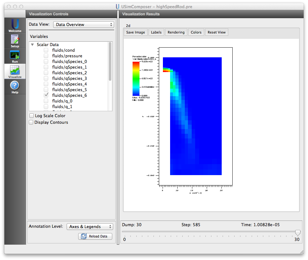
Figure 94: Visualization of the electrons density for the Flow over a Cylindrical Rod example

Further experiments¶

Four Gmsh fomat mesh files are included with this example, the default (highSpeedRod.msh), which is a low-resolution mesh that is partitioned for serial execution, versions of this mesh that is partioned so that it can be run with 2 (highSpeedRod2.msh), 4 (highSpeedRod4.msh) or 8 ((`highSpeedRod8.msh) cores along with a high resolution mesh that is partioned for either two (highSpeedRodHghRes2core.msh) or 24 (highSpeedRodHghRes24core.msh) cores. To run the example using this moderate resolution mesh on 2 cores, proceed as follows:

• Return to the “Setup” window by pressing the Setup button in the left column of buttons.
• Enter the mesh file name highSpeedRod2.msh next to meshFile.
• Press the Save And Process Setup button in the upper right corner.
• Proceed to the run window as instructed by pressing the Run button in the left column of buttons.
• In the “Run” window, press the MPI button in the left pane.
• Check the box marked Run with MPI and set Number of Cores equal to 2 as pictured in Fig. 95.

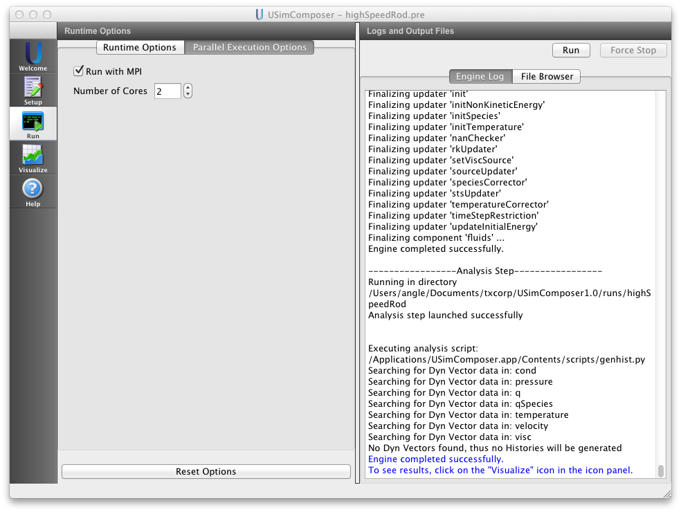
Figure 95: Run window showing the parallel option.

After setting the Number of Cores, run the simulation:

• To run the file, click on the Run button in the upper right corner. of the window. You will see the output of the run in the right pane. The run has completed when you see the output, “Engine completed successfully.”

After the simulation has executed, continue as follows:

• Proceed to the Visualize window as instructed by pressing the Visualize button in the left column of buttons.
• Press the “Open” button to begin visualizing.
• To visualize the geometry, expand the geometry tab and click the checkbox for fluids/domain.
• To visualize the electron density, expand the Scalar Data tab and click the check box for fluids/qSpecies_6.
• Drag the slider at the bottom of the visualization window to move through the simulation in time.