Supersonic Crossflow over a Cylinder (mach2Cylinder.pre)¶

Problem description¶

This simulation shows the supersonic flow over a cylinder. The formation of bow shock and the final steady wake can be seen in this laminar flow simulation. Full Navier-Stokes equations are used. Laminar flow assumption is used. Unstructured grid is used here. This grid was generated using gmsh. The convective and viscous parts are fully decoupled i.e the flow can be changed to inviscid by removing the viscous terms from the integration Updater. The properties of the fluid varying with temperature are computed within the input file. In this example, Sutherland’s formulas are used to obtain viscosity and thermal conductivity. The specific heats are assumed constant. Note that, the grid used in demonstrating this example is way coarse to display initial vortex shedding.

This simulation can be performed using USimHS license.

Creating the run space¶

The Supersonic Crossflow over a Cylinder example is accessed from within USimComposer by the following actions:

• Select the New from Template menu item in the File menu.
• In the resulting New from Template dialog, expand USimHS: Hypersonics.
• Select Supersonic Crossflow over a Cylinder and press the Choose button.
• In the Choose a name for the new runspace dialog, press the Save button to create a copy of this example in your run area.
• Press the Save And Process Setup button in the upper right corner of the Editor pane.

The basic example variables are editable in the Editor pane of the Setup window. After any change is made, the Save and Process Setup button must be pressed again before a new run commences.

Input file features¶

The following parameters can be varied:

• CFL - CFL condition for the simulation
• ATOMIC_MASS - Atomic mass of the gas
• GAS_GAMMA - Specific heat ratio of the gas
• RHO0 - Free stream density of the gas
• P0 - Free stream pressure of the gas
• U0 - Free stream velocity of the gas x-component
• V0 - Free stream velocity of the gas y-component
• SURFACE_TEMP - Surface temperature of the body
• CHARACTERISTIC_LENGTH - Characteristic length of the body
• MU_REF - Dynamic viscosity of the free stream gas
• SUTHERLAND - Sutherland coefficient
• TEMP_REF - Reference temperature in Sutherland’s formula
• TSTART - Simulation start time (seconds).
• TEND - Simulation end time (seconds).
• NUMDUMPS - Number of data dumps during the simulation
• GRIDFILE - Name of grid file
• DECOMPOSE - Type true for triangle and tetrahedral, false for 1d, quadrilateral and hexahedral
• CYLINDER_RADIUS - Radius of the cylinder
• X_MIN - Bottom left x-coordinate of the grid
• Y_MIN - Bottom left y-coordinate of the grid
• X_MAX - Top right x-coordinate of the grid
• Y_MAX - Top right y-coordinate of the grid

Note that the input file comes with an externally generated unstructured mesh using Gmsh. The parameters CYLINDER_RADIUS, (X_MIN,Y_MIN), and (X_MAX,Y_MAX) can be changed to accommodate a new mesh generated using Gmsh. The cylinder’s center is at origin.

Running the simulation¶

After performing the above actions, continue as follows:

• Proceed to the Run window as instructed by pressing the Run icon in the workflow panel.
• To run the simulation, click on the Run button in the upper right corner of the Logs and Output Files pane.

You will also see the engine log output in the Logs and Output Files pane. The run has completed when you see the output, “Engine completed successfully.”

Visualizing the results¶

After performing the above actions, continue as follows:

• Proceed to the Visualize window as instructed by pressing the Visualize icon in the workflow panel.
• Press the Open button to begin visualizing.
• Expand Geometries in the Visualization Controls pane and click the checkbox for fluids/domain to visualize simulation geometry.
• Expand Scalar Data and click the check box for fluids/temperature to visualize the temperature distribution.
• Drag the slider at the bottom of the Visualization Results pane to move through the simulation in time. The final distribution is shown in Fig. 96.

The conservative parameters density, three components of momentum, and energy can also be visualized using q_0,q_1,..,q_5 respectively. source_0 to source_3 represent the viscous sources of momentum and energy equations.

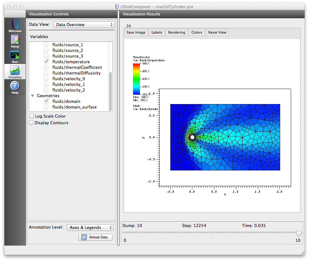
Figure 96: Visualization of temperature distribution in the Supersonic Crossflow over a Cylinder example

Further experiments¶

• Change the flow speed: For example increase U0 to 13600 (Mach 4) keeping the other flow parameters unchanged. Follow the steps and complete the simulation. The rise in shock temperature can be observed from the temperature distribution in the visualization window.
• Parallel: In the current version of USim, pre-partitioned unstructured mesh has to be used to run in parallel. The input file folder has partitioned mesh files for 2, 4, and 8 cores. (mach2CylinderQuad2.msh, mach2CylinderQuad4.msh, mach2CylinderQuad8.msh).