Point Source Volume Tally
Keywords:
-
radiation, GORAD
Problem Description
This problem illustrates how to set up a point source with an isotropic distribution within an angular range, measuring the energy deposited on a sphere and calculating fluence on a mesh.
Opening the Simulation
The Point Source Volume Tally example is accessed RSim by the following actions:
- Select the New → From Example… menu item in the File menu.
- In the resulting Examples window expand the RSim for Basic Radiation option.
- Expand the Basic Examples option.
- Select Point Source Volume Tally and press the Choose button.
- In the resulting dialog, create a New Folder if desired, and press the Save button to create a copy of this example.
All of the properties and values that create the simulation are now available in the Setup Window as shown in Fig. 63. You can expand the tree elements and navigate through the various properties, making any changes you desire. The right pane shows a 3D view of the geometry, if any, as well as the grid, if actively shown.
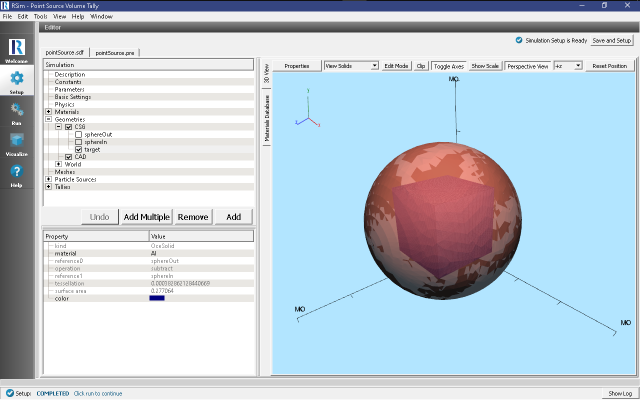
Fig. 63 Setup Window for the point particle source example.
Simulation Properties
This example demonstrates two physics features, and how CSG can be incorporated into RSim Simulations.
Under the Basic Settings tab the number of events to be simulated can be selected.
The particle source selected is a point shooting electrons. It shoots particles on a monoenergetic spectrum from zero to forty five degrees on the Z axis at an energy of 100.0 MeV.
Running the Simulation
After performing the above actions, continue as follows:
- Proceed to the Run Window by pressing the Run button in the left column of buttons.
- To run the file, click on the Run button in the upper left corner of the Logs and Output Files pane. You will see the output of the run in the right pane. The run has completed when you see the output, “Engine completed successfully.” This is shown in Fig. 64.
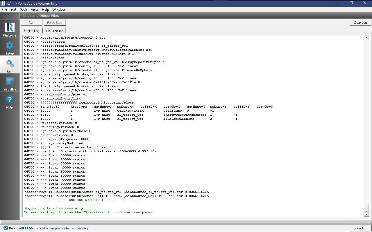
Fig. 64 The Run Window at the end of execution.
Visualizing the Results
After the simulation is completed it is possible to visualize the sphere and the total energy depostion on the sphere as shown in Fig. 65.
To view this
- Expand Scalar Data
- Check EnergyDepositOnSphere
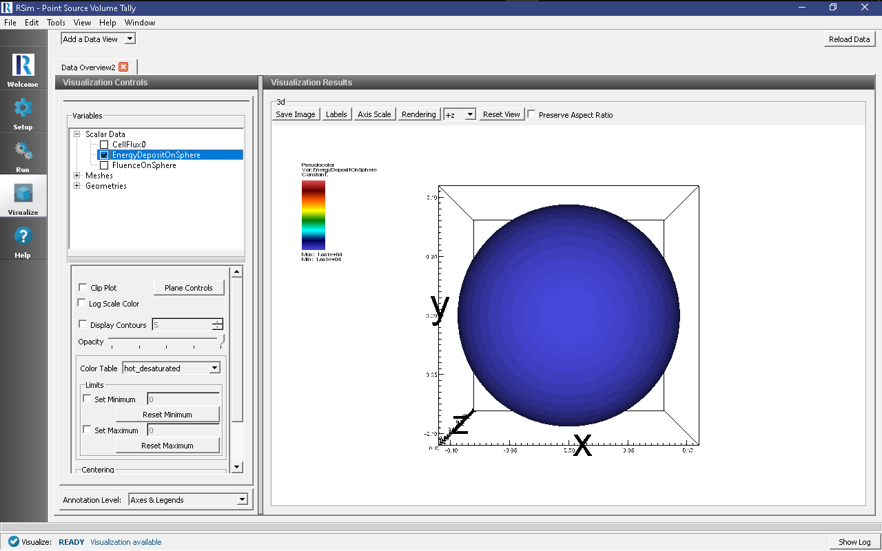
Fig. 65 The visualization window with results of the volume tally.
On a different data view
- Expand Scalar Data
- Check CellFlux0
- Check the Clip Plot box, and select Plane Controls Setting the Clip Plane Normal to X
- Rotate the image 90 degrees to the left
- Check the Set Minimum box and set it to 0
- Check the Set Maximum box and set it to 2e3
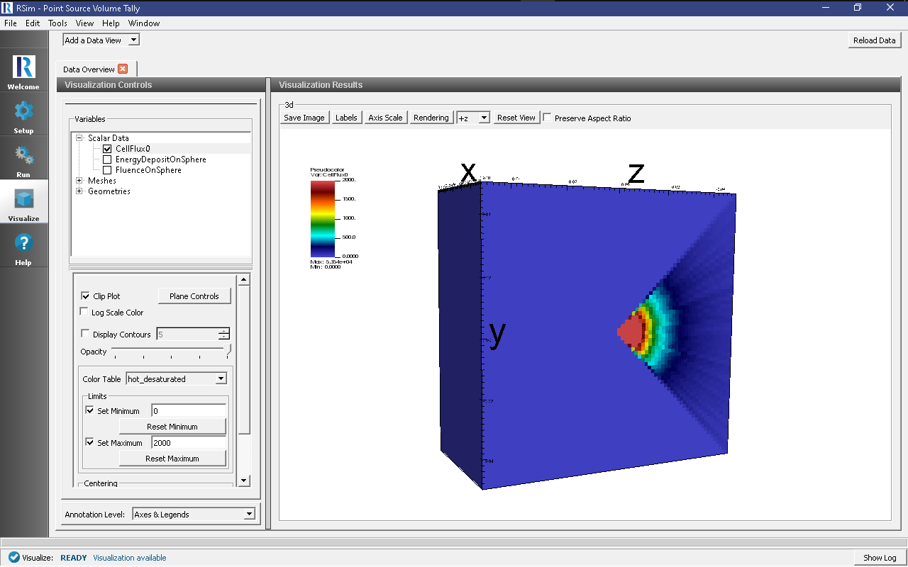
Fig. 66 The second visualization window with the results of the mesh tally.
Further Experiments
Try altering the particles used in the source or min and max angles in the source: for example using [0,180] range.