Proton Therapy

Problem Description

This problem illustrates a highly simplified version of proton therapy.

In this example a simplified human skeleton is modeled with a tumor embedded in adipose tissue and covered with skin on the back. A circular proton beam of 90 MeV energy is centered on the tumor. The energy deposited on the skin, fat, tumor and torso are all recorded.

For materials, the ICRP models built into RSim are used.

Opening the Simulation

The proton therapy example is accessed from within RSim by the following actions:

• Select the New → From Example… menu item in the File menu.
• In the resulting Examples window expand the RSim for Basic Radiation option.
• Expand the Basic Examples option.
• Select Proton Therapy and press the Choose button.
• In the resulting dialog, create a New Folder if desired, and press the Save button to create a copy of this example.

All of the properties and values that create the simulation are now available in the Setup Window as shown in Fig. 67. You can expand the tree elements and navigate through the various properties, making any changes you desire. The right pane shows a 3D view of the geometry, if any, as well as the grid, if actively shown.

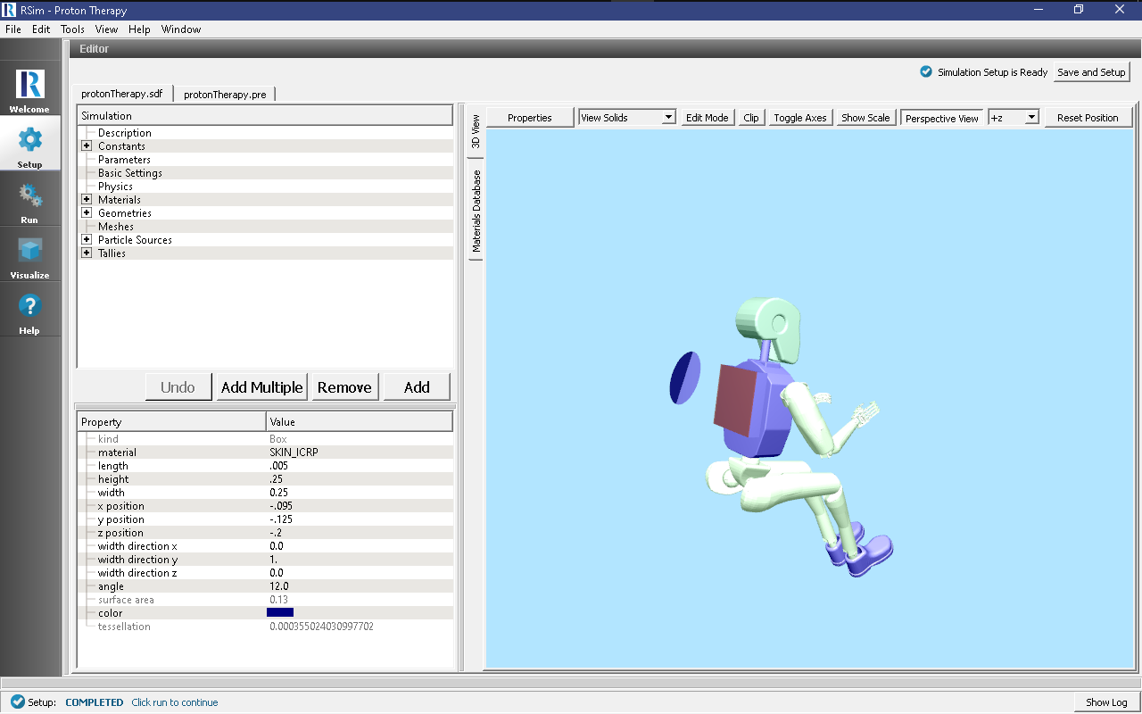
Fig. 67 Setup Window for the proton therapy example.

Simulation Properties

This example makes use of the Op 3 electromagnetics physics list, which is best for medical applications.

Under the Basic Settings tab the number of events to be simulated can be selected, as well as the number of threads to devote to the simulation.

The particle source selected is an elliptic plane. In this case it is a 1D Beam with 3 degrees of dispersion, and a monoenergetic energy distribution at 90 MeV.

Running the Simulation

After performing the above actions, continue as follows:

• Proceed to the Run Window by pressing the Run button in the left column of buttons.
• To run the file, click on the Run button in the upper left corner of the Logs and Output Files pane. You will see the output of the run in the right pane. The run has completed when you see the output, “Engine completed successfully.” This is shown in Fig. 68.

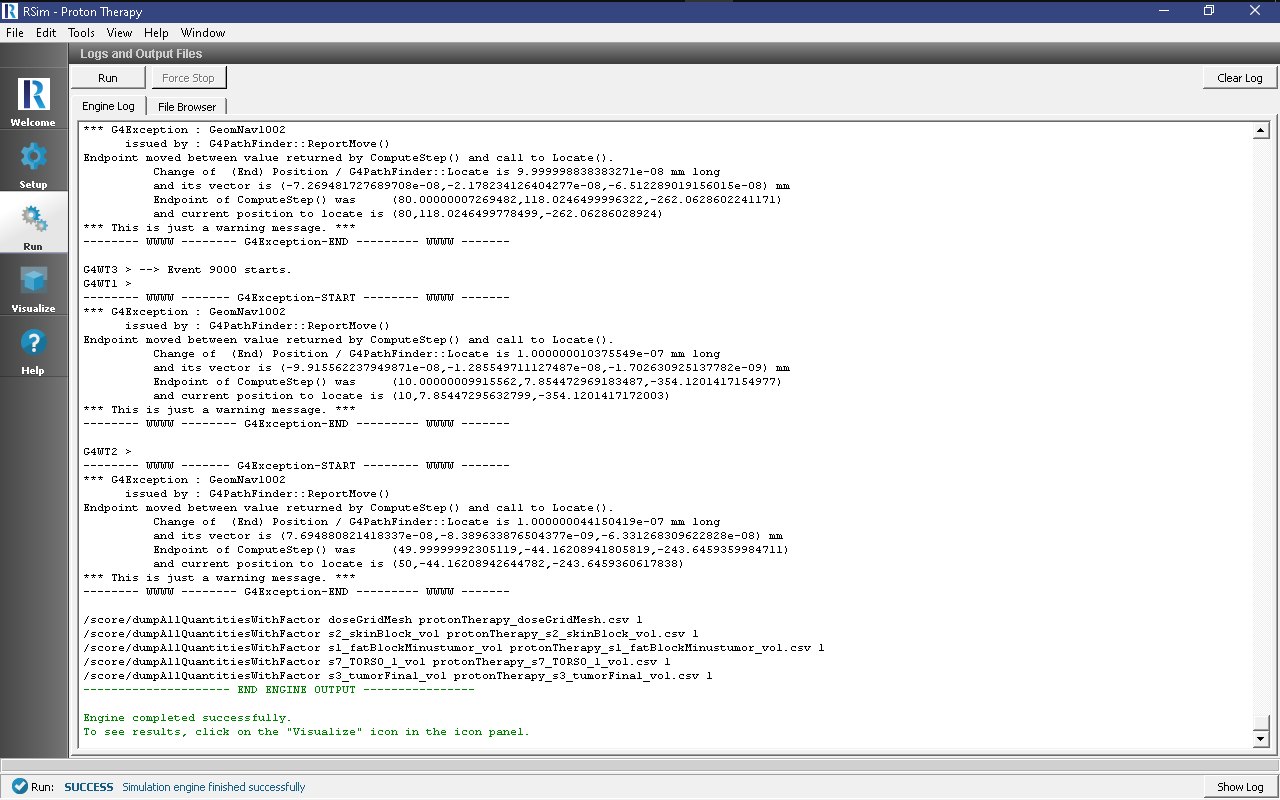
Fig. 68 The Run Window at the end of execution.

Visualizing the Results

After the simulation has completed, click on the Visualize button as shown in Fig. 69):

• Expand Scalar Data
• Check doseFat, doseSkeleton and doseSkin.

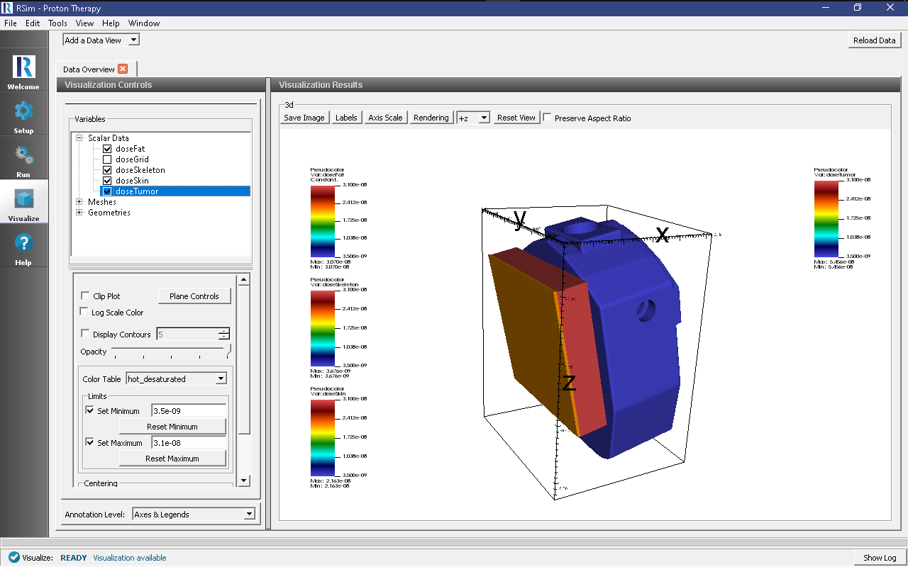
Fig. 69 The visualization results.

This can show how the dosage on the Fat is higher than that of the Skin or Skeleton.

In order to visualize tumor, it is better to see the mesh tally result.

• Click Add a Data View
• Choose Data Overview
• Expand Scalar Data
• Choose doseGrid
• Select the hot_and_cold color table
• Click on Clip Plots
• Click on Plane Controls
• Choose settings shown in Fig. 70:
• Expand *Geometries
• Click on *s7_TORSO_1
• Click on Clip Plots
• Click on Plane Controls
• Choose settings shown in Fig. 70:

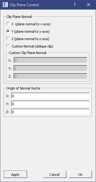
Fig. 70 Settings of the cut plane.

The resulting image shows the tumor deposit as shown in Fig. 71:.

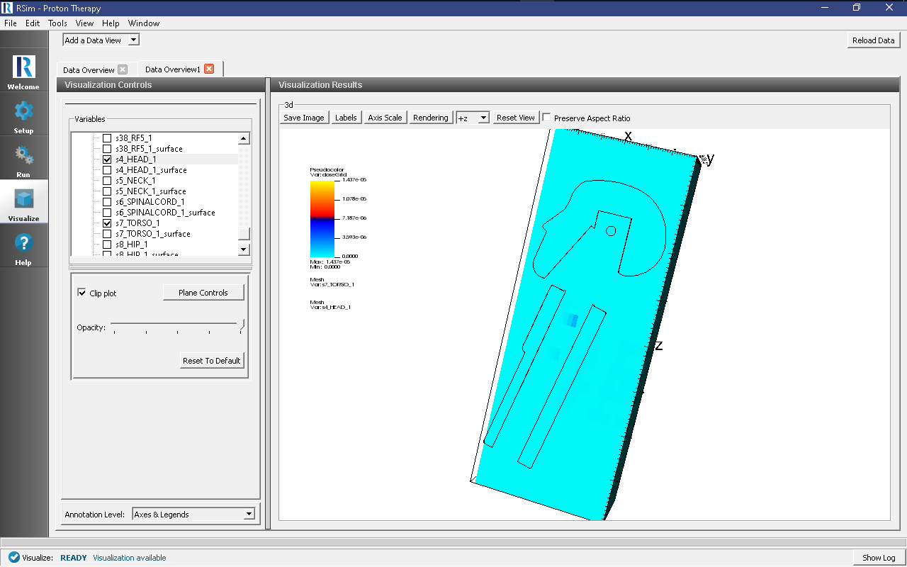
Fig. 71 The visualization of the volume tally.

Further Experiments

Try altering the energy of the beam to see an increase in the dose on the “tumor” or increasing the thickness of the fat block to see how it may reduce the ionizing dose.