Flow over a Forward-Facing Step (forwardFacingStep.pre)¶

Problem description¶

This problem demonstrates supersonic flow over a forward-facing step, involving Mach 3 flow at an inlet to a rectangular domain. A step is placed near the inlet region that generates shock waves. An unstructured mesh, with a reflecting wall boundary at the step, is used in this example.

This simulation can be performed with a USimBase license.

Creating the run space¶

The Flow over a Forward-Facing Step example is accessed from within USimComposer by the following actions:

• Select the New from Template menu item in the File menu.
• In the resulting New from Template dialog, expand USimBase: Basic Physics Capabilities.
• Select Flow over a Forward-Facing Step and press the Choose button.
• In the Choose a name for the new runspace dialog, press the Save button to create a copy of this example in your run area.
• Press the Save And Process Setup button in the upper right corner of the Editor pane.

The basic example variables are editable in the Editor pane of the Setup window as shown below. After any change is made, the Save and Process Setup button must be pressed again before a new run may commence.

Input file features¶

The input file allows the user to set a variety of problem parameters related to the physics, initial conditions, domain and solver used for the Flow over a Forward-Facing Step.

The following parameters control the physics:

• MHD = False,True selects whether to evolve the problem in the inviscid hydrodynamic limit (MHD = False) or the ideal magnetohydrodynamic limit (MHD = True).
• BETA controls the ratio of the gas pressure to the magnetic pressure for problems solved in the magnetohydrodynamic limit (i.e. when MHD = True).
• GAS_GAMMA sets the adiabatic index (ratio of specific heats) of the fluid.
• GRIDFILE Mesh file to use
• GRIDFORMAT Format of the mesh file (either ExodusII or Gmsh)

The following parameters the length of the simulation and data output:

• TEND sets the end time for the simulation.
• NUMDUMPS sets the number of data dumps during the simulation
• WRITE_RESTART = False,True tells USim to output data necessary to restart the simulation. If this parameter is set to False then the Restart at Dump Number functionality in the Standard tab under Runtime Options in the Run window will not be available.

The following parameters control the USim solvers used to evolve the simulation:

• TIME_ORDER = first,second,third,fourth sets the order of accuracy for the time-integration.
• DIFFUSIVE = False,True sets whether to use diffusive (but robust!) spatial integration schemes.
• DEBUG = False,True sets whether to output data for debugging a run. Warning: this will output A LOT of information!

Running the simulation¶

After performing the above actions, continue as follows:

• Proceed to the Run window as instructed by pressing the Run icon in the workflow panel.
• To run the simulation, click on the Run button in the upper right corner of the Logs and Output Files pane.

You will also see the engine log output in the Logs and Output Files pane. The run has completed when you see the output, “Engine completed successfully.”

Visualizing the results¶

After performing the above actions, continue as follows:

• Proceed to the Visualize window as instructed by pressing the Visualize icon in the workflow panel.
• Press the Open button to begin visualizing.
• Expand Geometries in the Visualization Controls pane and click the checkbox for fluids/forwardFacingStep to visualize simulation geometry.
• Expand Scalar Data and click the check box for fluids/density to visualize fluid densities.
• Drag the slider at the bottom of the Visualization Results pane to move through the simulation in time. The fluid density distribution at the end of the simulation is shown in Fig. 75.

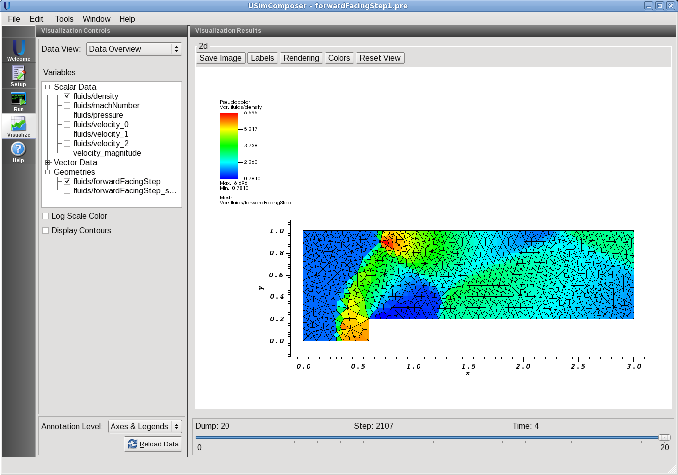
Figure 75: Visualization of the Flow over a Forward-Facing Step example using a color contour plot

Further experiments¶

Several Gmsh format mesh files are included with this example. The default file choice is “forwardFacingStep.msh”, which is a low-resolution mesh partitioned for serial execution. Higher-resolution meshes (forwardFacingStep2.msh, forwardFacingStep4.msh, forwardFacingStep8.msh) are included for 2, 4, and 8 core runs, respectively. To run the example using the 2-core mesh, proceed as follows:

• Return to the Setup window by pressing the Setup icon in the workflow panel.
• Enter the mesh file name “forwardFacingStep2.msh” in the GRIDFILE text box.
• Proceed to the Run window as instructed by pressing the Run icon in the workflow panel.
• In the Run window, press the MPI tab in the Runtime Options pane.
• Check the box marked Run with MPI and set Number of Cores equal to 2.
• To run the simulation, click on the Run button in the upper right corner of the Logs and Output Files pane. You will again see the engine output in the Logs and Output Files pane`.

After the simulation has executed, continue as follows:

• Proceed to the Visualize window as instructed by pressing the Visualize icon in the workflow panel.
• Press the Open button to begin visualizing.
• Expand Geometries in the Visualization Controls pane and click the checkbox for fluids/forwardFacingStep to visualize simulation geometry.
• Expand Scalar Data and click the check box for fluids/density to visualize fluid densities.
• Drag the slider at the bottom of the Visualization Results pane to move through the simulation in time.