Rayleigh-Taylor Instability (rtInstability.pre)¶

Problem description¶

This problem demonstrates the Rayleigh-Taylor instability for the case of a heavy fluid on top of a lighter fluid, subject to a constant gravitational acceleration. The pressure is determined by the conditions of hydrostatic equilibrium. For the two-dimensional version of the problem setup considered here, we use a domain

\((-TRANS_{LENGTH}/2,-PAR_{LENGTH}/2) \times (TRANS_{LENGTH}/2,PAR_{LENGTH}/2)\)

with periodic boundary conditions in the TRANS direction and reflecting wall boundary conditions in the PAR direction. For the three-dimensional version of the problem setup considered here, we use a domain

\((-TRANS_{LENGTH}/2,-PAR_{LENGTH}/2,-TRANS_{LENGTH}/2) \times (TRANS_{LENGTH}/2,PAR_{LENGTH}/2,TRANS_{LENGTH}/2)\)

with periodic boundary conditions in the TRANS directions and reflecting wall boundary conditions in the PAR direction. A single mode perturbation is used to seed the instability.

This simulation can be performed with a USimBase license.

Creating the run space¶

The Rayleigh-Taylor Instability example is accessed from within USimComposer by the following actions:

• Select the New from Template menu item in the File menu.
• In the resulting New from Template dialog, expand USimBase: Basic Physics Capabilities.
• Select Rayleigh-Taylor Instability and press the Choose button.
• In the Choose a name for the new runspace dialog, press the Save button to create a copy of this example in your run area.
• Press the Save And Process Setup button in the upper right corner of the Editor pane.

The basic example variables are editable in the Editor pane of the Setup window as shown below. After any change is made, the Save and Process Setup button must be pressed again before a new run may commence.

Input file features¶

The input file allows the user to set a variety of problem parameters related to the physics, initial conditions, domain and solver used for the Rayleigh-Taylor instability.

The following parameters control the physics of the Rayleigh-Taylor instability:

• GRAVITY_ACCEL sets the acceleration due to gravity.
• RHO_LIGHT sets the density of the lighter fluid initially at the bottom of the domain.
• RHO_HEAVY sets the density of the heavier fluid initially at the top of the domain.
• GAS_GAMMA sets the adiabatic index (ratio of specific heats) of the fluid.
• PERTURB_AMP sets the strength of the perturbation seeding the instability.
• MHD = False,True selects whether to evolve the problem in the inviscid hydrodynamic limit (MHD = False) or the ideal magnetohydrodynamic limit (MHD = True).
• BETA controls the ratio of the gas pressure to the magnetic pressure for problems solved in the magnetohydrodynamic limit (i.e. when MHD = True). Note that, for strong enough magnetic fields (small enough BETA), the instability is stabilized.

The following parameters control the dimensionality, domain size and resolution of the simulation:

• NDIM = 2,3 selects whether to run the problem in two-dimensions or three-dimensions.
• PAR_LENGTH sets the size of the domain in the direction parallel to the gravitational acceleration vector.
• TRANS_LENGTH sets the size of the domain in the direction transverse to the gravitational acceleration vector.
• PAR_ZONES sets the number of zones in the direction parallel to the gravitational acceleration vector.
• TRANS_ZONES sets the number of zones in the direction transverse to the gravitational acceleration vector.

The following parameters the length of the simulation and data output:

• TEND sets the end time for the simulation
• NUMDUMPS sets the number of data dumps during the simulation
• WRITE_RESTART = False,True tells USim to output data necessary to restart the simulation. If this parameter is set to False then the Restart at Dump Number functionality in the Standard tab under Runtime Options in the Run window will not be available.

The following parameters control the USim solvers used to run the simulation:

• TIME_ORDER = first,second,third,fourth sets the order of accuracy for the time-integration.
• DIFFUSIVE = False,True sets whether to use diffusive (but robust!) spatial integration schemes.
• DEBUG = False,True sets whether to output data for debugging a run. Warning: this will output A LOT of information!

Running the simulation¶

After performing the above actions, continue as follows:

• Proceed to the Run window as instructed by pressing the Run icon in the workflow panel.
• To run the simulation, click on the Run button in the upper right corner of the Logs and Output Files pane.

You will also see the engine log output in the Logs and Output Files pane. The run has completed when you see the output, “Engine completed successfully.”

Visualizing the results¶

After performing the above actions, continue as follows:

• Proceed to the Visualize window as instructed by pressing the Visualize button in the left column of buttons.
• Press the “Open” button to begin visualizing.
• To visualize the fluid density, expand the Scalar Data tab and click the check box for fluids/density.
• Drag the slider at the bottom of the visualization window to move through the simulation in time. The fluid density distribution at the end of the simulation is shown in Fig. 78.

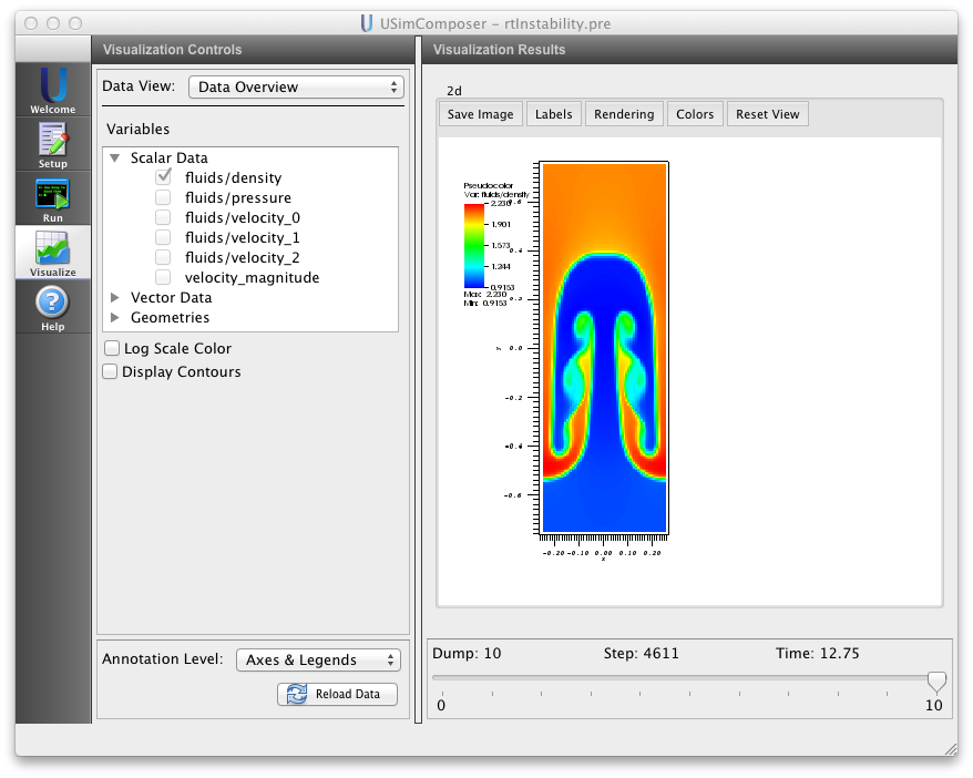
Figure 78: Visualization of density in the Rayleigh-Taylor instability example as a color contour plot.

Further experiments¶

• Set MHD to True to solve the magnetized Rayleigh-Taylor instability.
• Set TIME_ORDER to third or fourth to see the effect of increased temporal accuracy on the Rayleigh-Taylor instability.
• Set NDIM to 3 to solve the Rayleigh-Taylor instability in 3D. The increased computational requirements of such a simulation means that you should enable Run with MPI in the MPI tab under Runtime Options in the Run Window.