Diffusion (diffusion.pre)¶

Problem description¶

This example models thermal diffusion from a cylindrical wall held at constant temperature. The diffusion scheme here can be used for all types of diffusion including thermal and species diffusion. This example uses the super time stepping integrator which accelerates the solution of diffusion type systems compared to standard explicit approaches.

This simulation can be performed with USimHS and USimHEDP license.

Creating the run space¶

The Diffusion example is accessed from within USimComposer by the following actions:

• Select the New from Template menu item in the File menu.
• In the resulting New from Template dialog, expand USimHS: Hypersonics.
• Select Diffusion and press the Choose button.
• In the Choose a name for the new runspace dialog, press the Save button to create a copy of this example in your run area.
• Press the Save And Process Setup button in the upper right corner of the Editor pane.

The basic example variables are editable in the Editor pane of the Setup window. After any change is made, the Save and Process Setup button must be pressed again before a new run commences.

Input file features¶

The input folder has externally generate mesh file using Gmsh. The following parameters can be varied to simulate different flow regimes.

• GRIDFILE - Name of grid file
• NUMDUMPS - Number of data dumps during the simulation
• EXPLICIT_CFL - the explicit CFL to use to compute the number of STS cycles
• STS_CFL - the actual CFL
• USESTS - is 1 if the STS method is used 0 if the standard explicit approach should be used

Running the simulation¶

After performing the above actions, continue as follows:

• Proceed to the Run window as instructed by pressing the Run icon in the workflow panel.
• To run the simulation, click on the Run button in the upper right corner of the Logs and Output Files pane.

You will also see the engine log output in the Logs and Output Files pane. The run has completed when you see the output, “Engine completed successfully.”

Visualizing the results¶

After performing the above actions, continue as follows:

• Proceed to the Visualize window as instructed by pressing the Visualize icon in the workflow panel.
• Press the Open button to begin visualizing.
• Expand Scalar Data and click the check box for fluids/q to get the temperature distribution.
• Drag the slider at the bottom of the Visualization Results pane to move through the simulation in time. The temperature distribution at the end of the simulation is shown in Fig. 92.

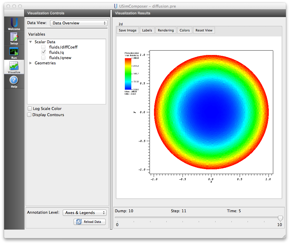
Figure 92: Visualization of thermal diffusion.

Further experiments¶

• Switch USESTS to 0 to see how much slower the simulation runs when standard explicit methods are used.
• Increase STS_CFL to see how the solution changes as larger and larger time steps are used.