Cylindrical Capacitor (cylindricalCapacitor.sdf)
Keywords:
- cylindrical, capacitor, electrostatic
Problem description
The Cylindrical Capacitor simulation solves for the potential between two cylinders with a ring of charge.
This simulation can be performed with a VSimBase license.
Opening the Simulation
The Cylindrical Capacitor example is accessed from within VSimComposer by the following actions:
Select the New → From Example… menu item in the File menu.
In the resulting Examples window expand the VSim for Basic Physics option.
Expand the Basic Examples option.
Select Cylindrical Capacitor and press the Choose button.
In the resulting dialog, create a New Folder if desired, and press the Save button to create a copy of this example.
All of the properties and values that create the simulation are
now available in the Setup Window as shown in
Fig. 151. You can expand the tree
elements and navigate through the various properties, making any
changes you desire. The right pane shows a 3D view of the
geometry, if any, as well as the grid, if actively shown. To show
or hide the grid, expand the Grid element and select or deselect
the box next to Grid.
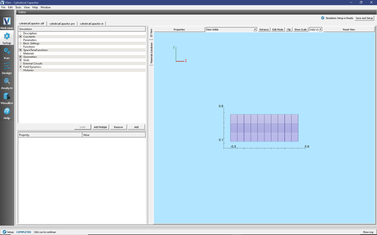
Fig. 151 Setup Window for the Cylindrical Capacitor example.
Simulation Properties
In this simulation there is a backgroundChargeDensity0 field which is given by an expression, chargedDist. That expression is defined as a SpaceTimeFunction. The variables x and y in the expression are place holders for the actual variables, Z and R, in the simulation. So this is a ring of charge, centered at R = 0.3, with a Gaussian fall off.
There are Dirichlet boundary conditions on the lower and upper R boundaries, with the lower bound set to 10 volts.
Running the simulation
After performing the above actions, continue as follows:
Proceed to the Run Window by pressing the Run button in the left column of buttons.
Here you can set run parameters and the run mode (serial or parallel)
When you are finished setting run parameters, click on the Run button in the upper left corner of the window. You will see the output of the run in the right pane. The run has completed when you see the output, “Engine completed successfully.” This is shown in Fig. 152.
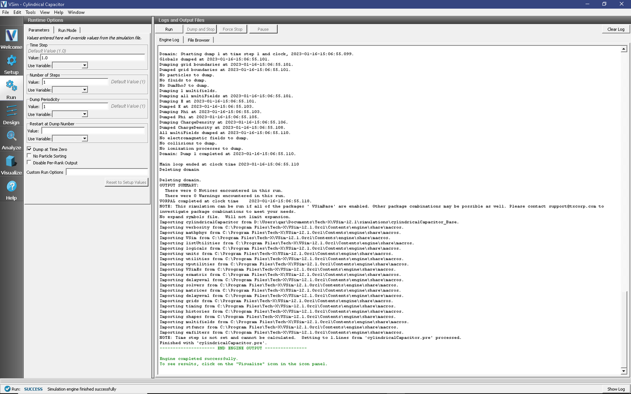
Fig. 152 The Run Window at the end of execution.
Visualizing the results
After performing the above actions, continue as follows:
Proceed to the Visualize Window by pressing the Visualize button in the left column of buttons.
This particular run computes the electrostatic potential, which we see by opening the scalar data and checking the box next to Phi, which is shown in the right of the visualization tab. See Fig. 153.
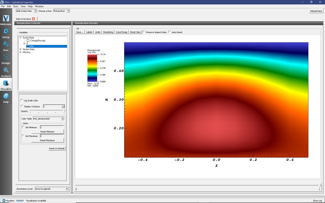
Fig. 153 Visualization of the electrostatic potential
Further Experiments
Looking inside the field boundary conditions, and highlighting dirichlet0, you can see that 10V was put on the lower R boundary. You can try experimenting with this, going to run and visualize with each change. The more voltage, the less the background charge should matter.
You can take the charge out of the system. Highlight the backgroundChargeDensity0 label. In the property editor below, double click on chargedDist, hit delete, and type 0.0. Then run and viz, and you will see a potential that is independent of Z.
Click the Add a Data View dropdown below the menu bar and select Field Analysis. For the Field, choose E_r with the Vertical Lineout Settings, then hit “Perform Lineout”. You will see, as expected, that the radial electric field is positive (pointing outward) and falling off with the expected 1/r behavior.