Vacuum Electromagnetic Pulse (emPulseInVacuum.sdf)
Keywords:
- electromagnetics, laser, plane wave pulse, field energy monitoring
Problem description
A linearly-polarized (with electric field in the z-direction) electromagnetic pulse with a sinusoidal amplitude on a plane wave is launched from the left side (x=0). The transverse (y, z) boundary conditions are periodic, but the pulse has finite transverse extent.
This simulation can be performed with a VSimBase license.
Opening the Simulation
The Vacuum Electromagnetic Pulse example is accessed from within VSimComposer by the following actions:
Select the New → From Example… menu item in the File menu.
In the resulting Examples window expand the VSim for Basic Physics option.
Expand the Basic Examples option.
Select Vacuum Electromagnetic Pulse and press the Choose button.
In the resulting dialog, create a New Folder if desired, and press the Save button to create a copy of this example.
All of the properties and values that create the simulation are now available
in the Setup Window as shown in Fig. 163.
You can expand the tree elements and navigate through the
various properties, making any changes you desire. The right pane shows a 3D
view of the geometry, if any, as well as the grid, if actively shown. To show
or hide the grid, expand the Grid element and select or deselect the box next
to Grid.
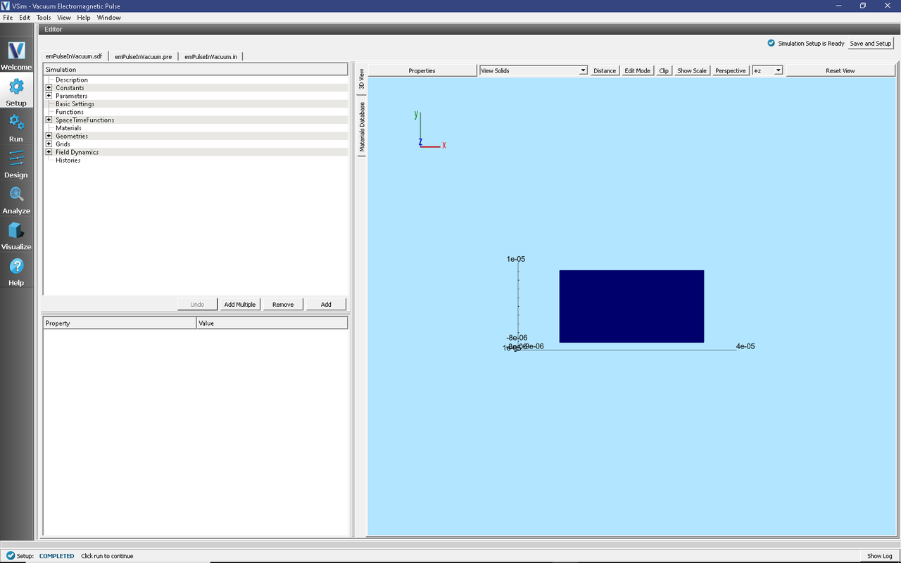
Fig. 163 The Setup Window for the electromagnetic pulse.
Simulation Properties
The Vacuum Electromagnetic Pulse example includes several constants for easy adjustment of simulation properties. Those include:
AMPLITUDE: The amplitude of the pulse
WAVELENGTH: The wavelength of the pulse
PULSELENGTH: The length of the pulse in the propagation direction
PULSEWIDTH: The width of the pulse in the transverse direction
There is also a SpaceTimeFunction defined for the pulse shape and is used in the Port Launcher boundary condition.
Running the Simulation
After performing the above actions, continue as follows:
Proceed to the Run Window by pressing the Run button in the left column of buttons.
To run the file, click on the Run button in the upper left corner of the Logs and Output Files pane. You will see the output of the run in the right pane. The run has completed when you see the output, “Engine completed successfully.”
The Run Window, showing settable parameters with the engine output in the right pane, is shown in Fig. 164.
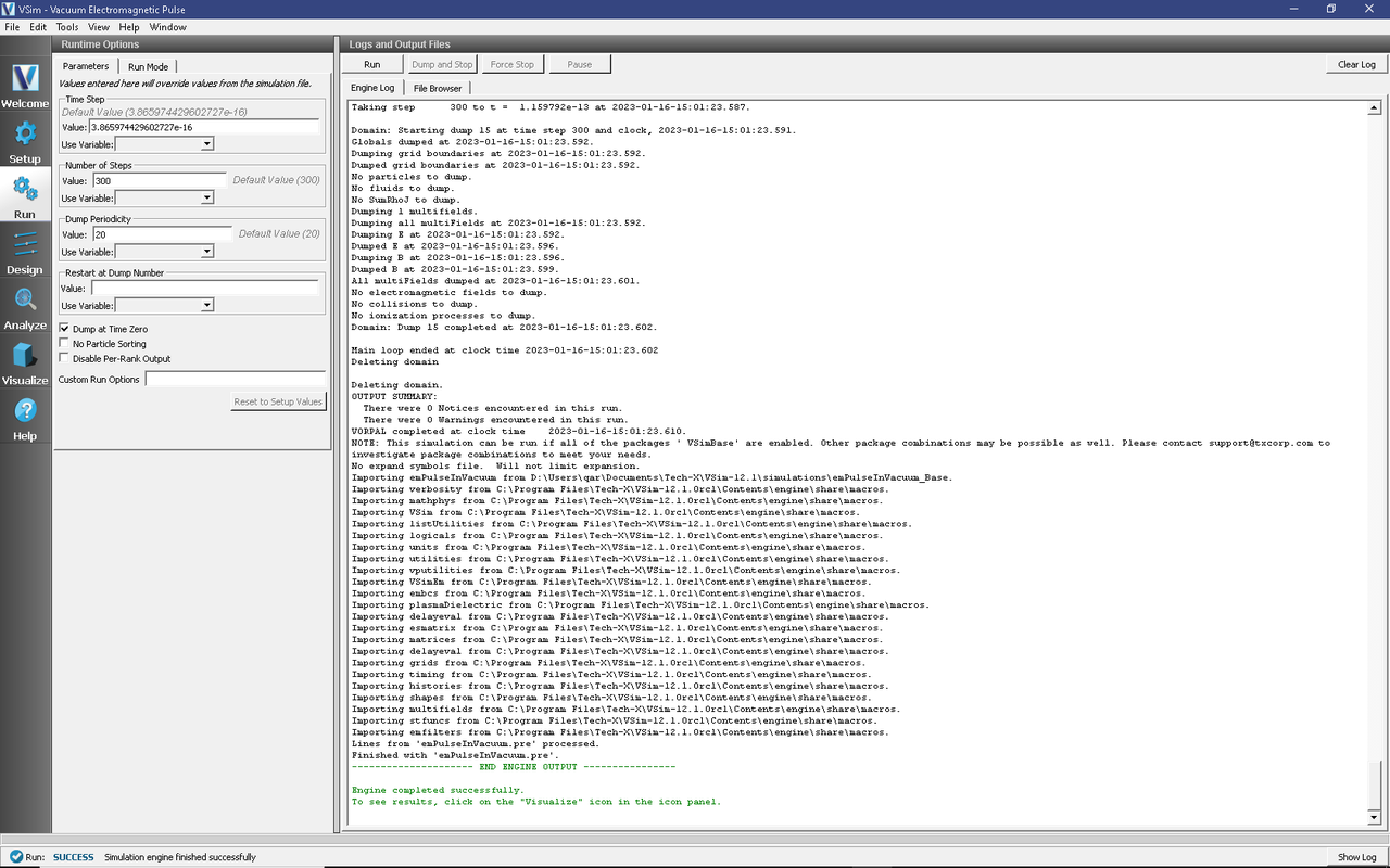
Fig. 164 The Run Window for the electromagnetic pulse.
Visualizing the Results
After performing the above actions, continue as follows:
Proceed to the Visualize Window by pressing the Visualize button in the left column of buttons.
The electric and magnetic field components can be found in the scalar data variables of the data overview tab.
Make sure the Data View drop down is set to Data Overview.
Here you can see Variables. Expand the Scalar Data.
Expand E
Select E_z
Check the box next to Clip Plot
Check the box next to Display Contours and set the # of contours to 5
Click and drag with your mouse to rotate the view
Initially, no field will be seen, as one is looking at Dump 0, the initial dump, when no fields are yet in the simulation. Move the slider at the bottom of the right pane to see the magnetic field at different times.
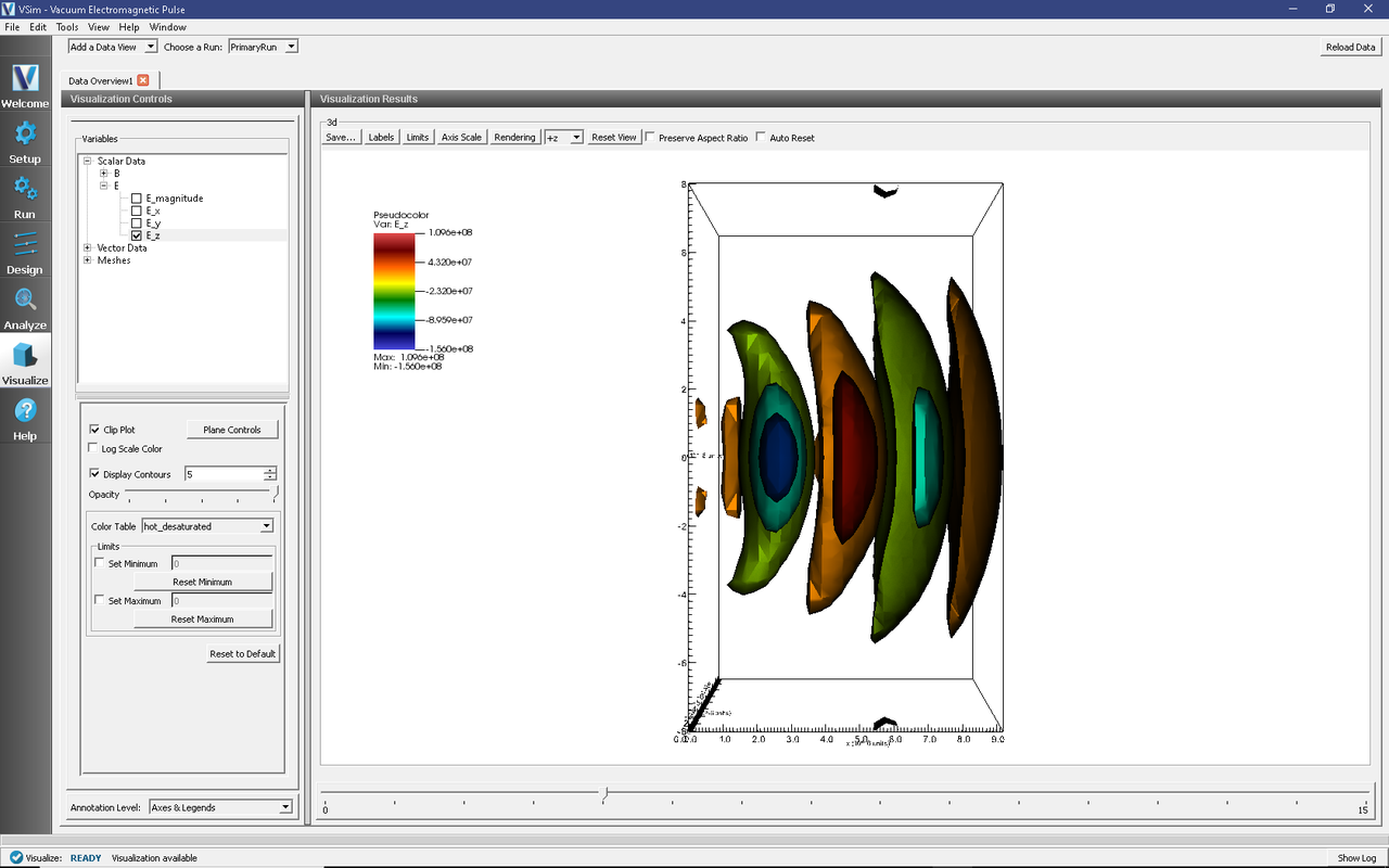
Fig. 165 Ez field at Dump 5.
Further Experiments
Increase NX to better resolve the wave and see whether it slips less with respect to the box.
Increase the pulse and box widths (you will also need to increase the number of cells in the transverse directions) to reduce diffraction.