Dipole Antenna (dipoleAntenna.sdf)
Keywords:
- antenna, electromagnetics, current source
Problem Description
Dipole antennas are the simplest and most widely used type of antenna. In the most basic setup, a dipole antenna is composed of an oscillating current/voltage source in between two electrodes. The frequency of the source will determine the wavelength of the electromagnetic radiation emitted from the antenna according to the dispersion relation
Most commonly, the electrodes will be 1/4 of the emitted wavelength. In this example, the antenna will be driven with a current oscillating with a frequency of 1 GHz. Therefore, the emitted wavelength will be roughly 30 cm, meaning we will make each of the electrodes 7.5 cm. This will make the total length of the antenna 15 cm, which is why dipole antennas are sometimes called half-wave antennas. It is easiest to drive the antenna when the electrodes are a quarter wavelength.
For more background information on dipole antennas, visit the Wikipedia page: https://en.wikipedia.org/wiki/Dipole_antenna
This simulation can be run with a VSimEM, VSimVE, or VSimPD license.
Opening the Simulation
The Dipole Antenna example is accessed from within VSimComposer by the following actions:
Select the New → From Example… menu item in the File menu.
In the resulting Examples window expand the VSim for Electromagnetics option.
Expand the Antennas option.
Select Dipole Antenna and press the Choose button.
In the resulting dialog box, create a New Folder if desired, then press the Save button to create a copy of this example.
The resulting Setup Window is shown Fig. 207.
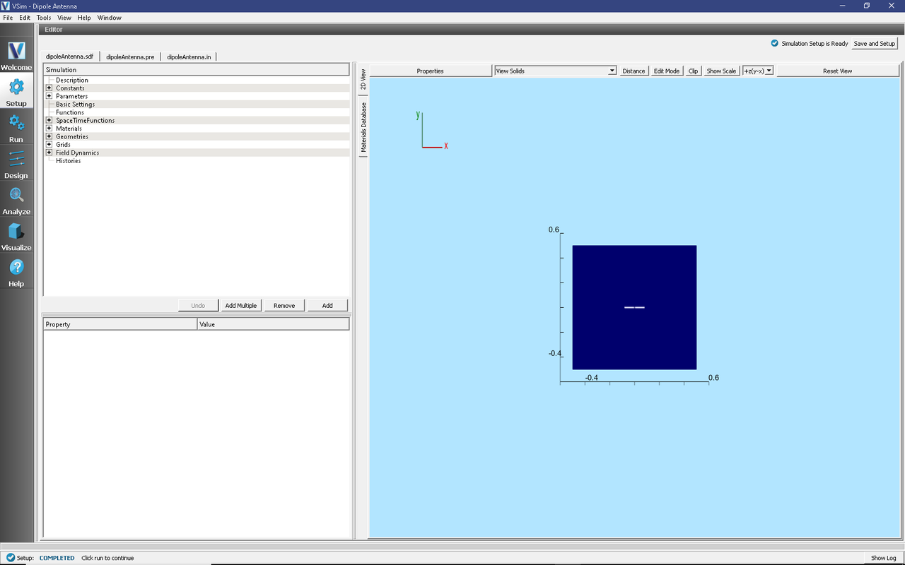
Fig. 207 Setup Window for the Dipole Antenna example.
Simulation Properties
In this simulation, we will excite the antenna and watch the dipole electromagnetic radiation emanate from the antenna. A distributed current source is used to apply the driving current. A volume for the current source and the functional form of the current is set under Field Dynamics \(\rightarrow\) CurrentDistributions \(\rightarrow\) DrivingCurrent. The user has the ability to set all three components of the current within the volume. In this example, we set the x-component of the current using the drivingCurrent spacetime function. The drivingCurrent function is a sine wave oscillating at 1 GHz to which a smooth turn on profile has been applied.
There are open boundaries on the walls of the simulation.
Running the Simulation
To run the simulation:
Proceed to the run window by pressing the Run button in the left column of buttons.
Here you can set run parameters, including how many cores to run with (under the MPI tab).
When you are finished setting run parameters, click on the Run button in the upper left corner. You will see the output of the run in the right pane.
The run has completed when you see the output, “Engine completed successfully.” This is shown in Fig. 208.
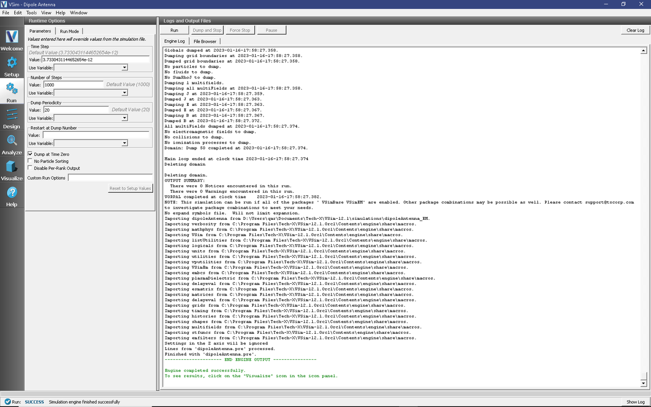
Fig. 208 The Run window at the end of execution.
Visualizing the Results
After performing the above actions, the results can be visualized as follows:
Proceed to the Visualize Window by pressing the Visualize button in the navigation column.
With the Data Overview open, expand Scalar Data then expand E.
Check the box for E_y. This will plot the y-component of the electric field.
For the color limits, set Set Minimum to -0.5, and Set Maximum to 0.5.
Scroll through the dumps to see how the y-component of the electric field changes with time. The last dump is shown in Fig. 209.
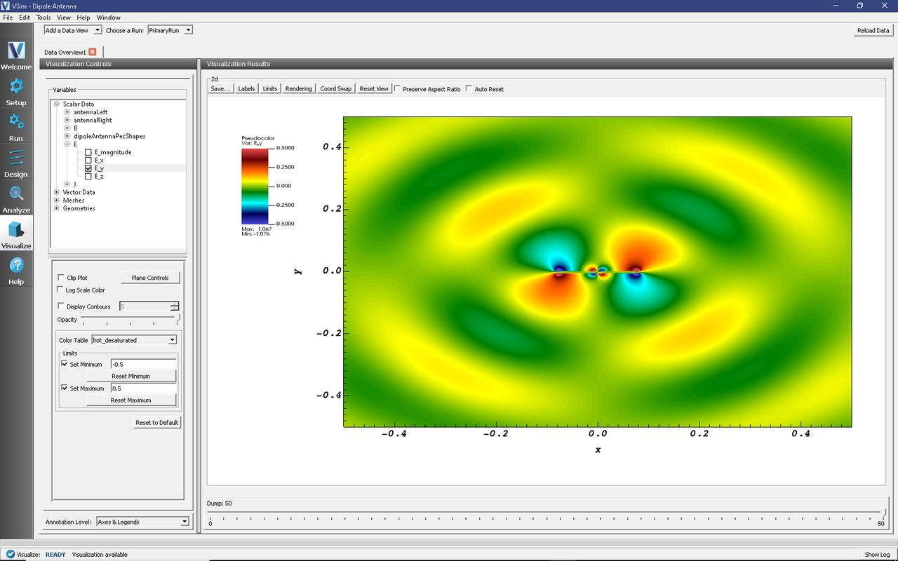
Fig. 209 The y-component of the Electric Field shows a 4-lobe pattern.
Un-check the E_y box, then check the box for E_magnitude. Then go back to the Colors Options and switch Set Minimum to -.1 and Set Maximum to 0.5. The magnitude of the electric field at the end of the simulation is shown in Fig. 210.
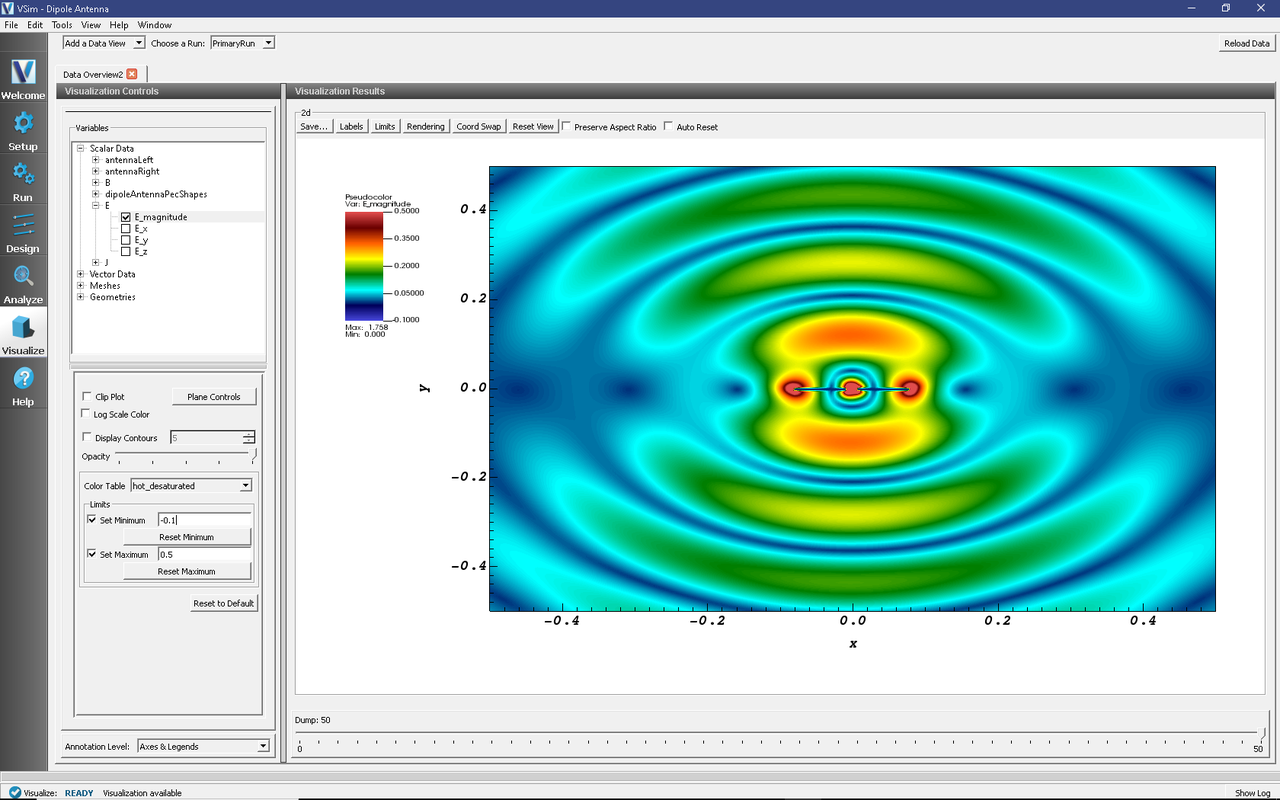
Fig. 210 The magnitude of the electric field shows the full 2-lobed dipole antenna pattern.
Further Experiments
Add an RCS Box around the antenna to measure the far field radiation pattern at a location of your choosing.
Modify the driving frequency or the dimensions of the electrodes.