Dish Antenna (dishAntenna.sdf)
Keywords:
- electromagnetics, antennas
Problem Description
The Dish Antenna simulation illustrates how to get the radiation pattern from a source in the presence of a complex shape.
This simulation can be performed with a VSimEM, VSimVE or VSimPD license.
Opening the Simulation
The Dish Antenna example is accessed from within VSimComposer by the following actions:
Select the New → From Example… menu item in the File menu.
In the resulting Examples window expand the VSim for Electromagnetics option.
Expand the Antennas option.
Select “Dish Antenna” and press the Choose button.
In the resulting dialog, create a New Folder if desired, and press the Save button to create a copy of this example.
All of the properties and values that create the simulation are now available in the Setup Window as shown in Fig. 215. You can expand the tree elements and navigate through the various properties, making any changes you desire. The right pane shows a 3D view of the geometry, if any, as well as the grid, if actively shown. To show or hide the grid, expand the Grid element and select or deselect the box next to Grid.
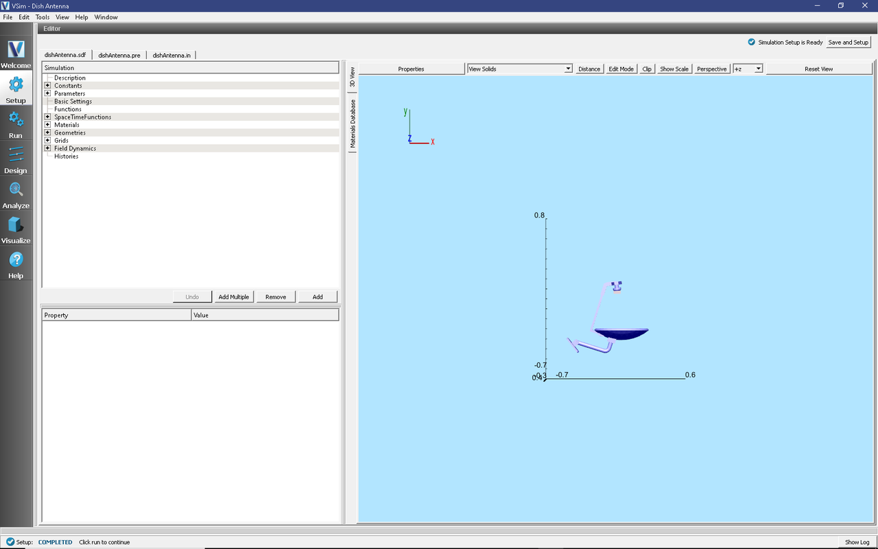
Fig. 215 Setup Window for the Dish Antenna example.
Simulation Properties
One can set the parameters of the grid and the source through the setup tree. The parameters are put under the Constants section.
Running the Simulation
After performing the above actions, continue as follows:
Proceed to the Run Window by pressing the Run button in the left column of buttons.
To run the file, click on the Run button in the upper left corner of the Logs and Output Files pane. You will see the output of the run in the Logs and Output Files pane. The run has completed when you see the output, “Engine completed successfully.” This is shown in Fig. 216.
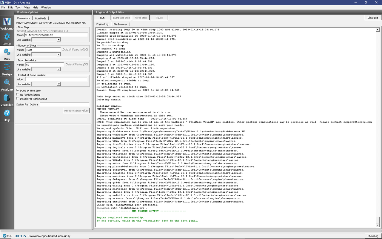
Fig. 216 The Run Window at the end of execution.
Visualizing the Results
After performing the above actions, continue as follows:
Proceed to the Visualize Window by pressing the Visualize button in the left column of buttons.
To view the electric field reflected from the dish antenna as shown in Fig. 217, do the following:
Expand Scalar Data
Expand E
Select E_x
Check Clip Plot
Expand Geometries
Select poly (dishAntennaPecShapes)
Check Clip Plot
It is easier to see the fields if you change the color scale minimum and maximum. To do so, check the Set Minimum and Set Maximum boxes, and set a fixed minimum of -2 and a fixed maximum of 2.
Move the slider at the bottom of the right pane to see the electric field at different times.

Fig. 217 Visualization of a slice of the electric field as a color contour plot at dump 19.
Further Experiments
Additional experiments worth investigating are:
Change the resolution to see whether more resolution gives a different answer.
Change the frequency of the source. Be careful, because at high frequencies with the chosen resolution, one will require a large amount of memory.