Dielectric in Electrostatics (dielectricInES.sdf)
Keywords:
- dielectric, electrostatics, capacitor
Problem Description
This simulation and the dielectricInEM demonstrate the differences between simulating dielectric materials with electrostatic and electromagnetic solvers. They also demonstrate some of the more general differences between electrostatic and electromagnetic simulations.
Both of these simulations represent the same physical system: a slab of dielectric between two metal plates. The simulation grid is one square meter with a .75m x .25m slab of dielectric centered between the plates. The electric potential and electric field are solved over the entire domain.
Electrostatics is an approximation of the full set of Maxwell’s equations. According to Faraday’s law,
In the electrostatic limit, fields change slowly. More precisely, \(\frac{\partial B}{\partial t} \approx 0\), so that any curling electric field is negligible compared to the full electric field. When curling electric fields can be neglected, the electric field is a conservative field and can be written as the gradient of a scalar function. This scalar function is the electric potential, or voltage, and satisfies Poisson’s equation
Electrostatics is appropriate if the shortest wavelength of interest, \(\lambda_{EM}\) is much longer than the length scale of the simulation \(L_{s}\). This criterion, \(\lambda_{EM} > L_s\) respects the “fields change slowly” heuristic. Divide both sides of the expression by the speed of light and we get that the period of an electromagnetic oscillation is longer than the time it takes light to cross the simulation domain. In this limit, any change to a field that occurs within a timestep will have time to propagate throughout the simulation domain within the same timestep.
As can be seen in Poisson’s equation, electrostatics does not respect relativity, since any change in \(\rho\) will instantaneously change the electric potential everywhere in the simulation. So, it is important to respect the \(\lambda_{EM} > L_s\) criterion when doing electrostatics, otherwise, the simulation might neglect some important physical effects.
This simulation can be run with a VSimEM, VSimVE, or VSimPD license.
Opening the Simulation
The Dielectric in Electrostatics example is accessed from within VSimComposer by the following actions:
Select the New → From Example… menu item in the File menu.
In the resulting Examples window expand the VSim for Electromagnetics option.
Expand the Electrostatics option.
Select Dielectric in Electrostatics and press the Choose button.
In the resulting dialog box, create a New Folder if desired, then press the Save button to create a copy of this example.
The resulting Setup Window is shown Fig. 248.
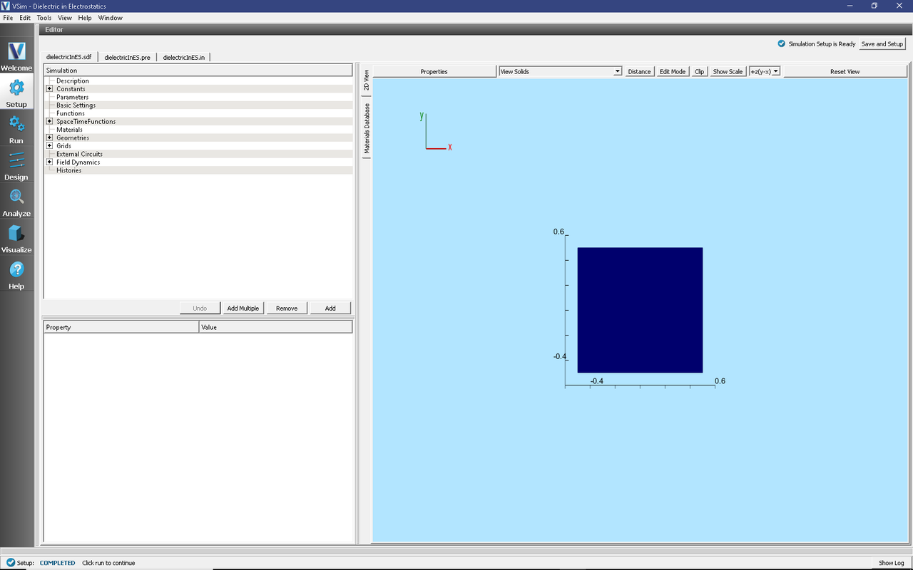
Fig. 248 Setup Window for the Dielectric in Electrostatics example.
Simulation Properties
In this simulation, voltages of 10.0 V and 0.0 V are set on the upper and lower boundaries (respectively) with Dirichlet boundary conditions. Neumann boundaries are used on the left and right walls of the simulation domain. In vacuum, this would set up an electric field of 10 V/m pointing down.
A dielectric is introduced to the simulation using a spacetime function
dielectricSapphire. Sapphire has a relative dielectric constant,
\(\epsilon_r = \frac{\epsilon_{sapphire}}{\epsilon_0},\) of 9.8.
Through the use of Heaviside functions, we set the relative permittivity
to be 9.8 in a rectangular region between \(x = \pm .375\) meters an
\(y = \pm .125\) meters and 1 everywhere else.
In the setup tree, the dielectricSapphire function is set as the
relative permittivity under Field Dynamics → PoissonSolver.
Running the Simulation
To run the simulation:
Proceed to the run window by pressing the Run button in the left column of buttons.
Here you can set run parameters, including how many cores to run with (under the MPI tab).
When you are finished setting run parameters, click on the Run button in the upper left corner. You will see the output of the run in the right pane.
The run has completed when you see the output, “Engine completed successfully.” This is shown in Fig. 249.

Fig. 249 The Run window at the end of execution.
Visualizing the Results
After performing the above actions, the results can be visualized as follows:
Proceed to the Visualize Window by pressing the Visualize button in the navigation column.
With the Data Overview tab open, expand Scalar Data then check the box for Phi.
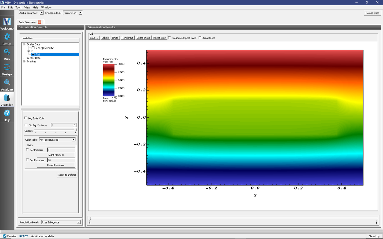
Fig. 250 The electric potential between the two parallel plates.
For a closer look at the potential, open the Field Analysis visualization tab by selecting it from the Add a Data View drop down menu at the very top right of the VSim Window.
In the new Field Analysis tab, from the Field drop down menu select “Phi.”
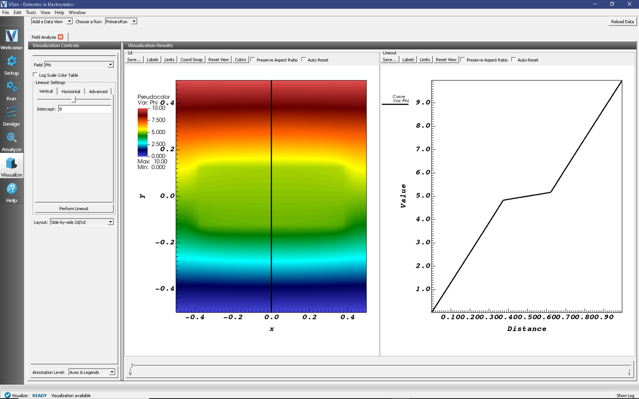
Fig. 251 Field Analysis tab showing the electric potential along the black vertical line.
The user can switch the location of the line out with the options on the left side of the screen.
Shown below is a plot with a horizontal line out at a position \(y = .18\) meters. Don’t forget to press the Perform Lineout button after adjusting the line out settings!
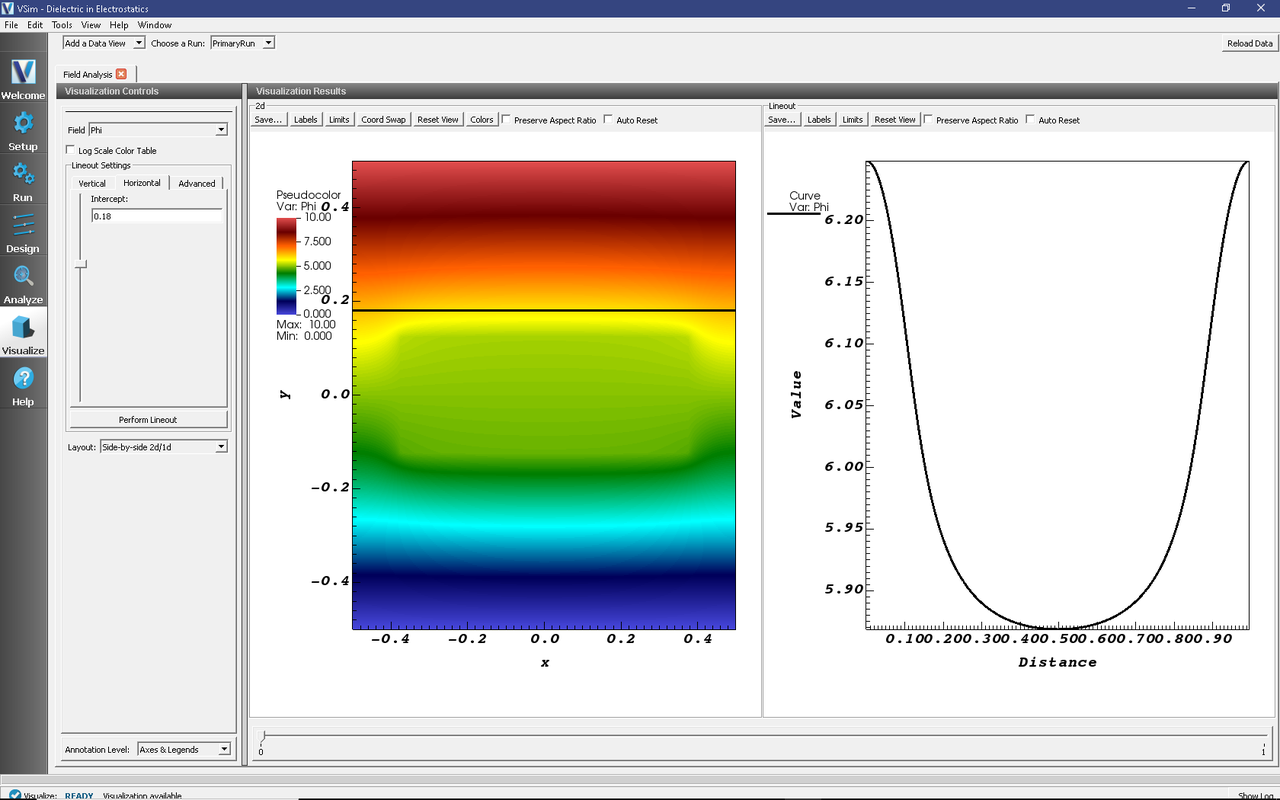
Fig. 252 Field Analysis tab showing line out in different position.
Further Experiments
Change the dielectric constant, or change the location and area of the dielectric. Add a sinusoidal voltage on the plates.