Specific Absorption Rate (humanHeadT.pre)
Keywords:
- dielectrics, power calculations, stl files
Problem Description
The Specific Absorption Rate simulation computes the power absorption in a human head where the brain tissue is approximated using a salt water model. A dipole source is included to imitate a simple antenna source from a cell phone. This example can serve as the basis for a true specific absorption rate calculation for a human head with a source coming from a cell phone antenna.
This simulation can only be performed with a VSimEM, VSimVE or VSimPD license.
Opening the Simulation
The Human Head example is accessed from within VSimComposer by the following actions:
Select the New → From Example… menu item in the File menu.
In the resulting Examples window expand the VSim for Electromagnetics option.
Expand the Other EM (text-based setup) option.
Select “Specific Absorption Rate (text-based setup)” and press the Choose button.
In the resulting dialog, create a New Folder if desired, and press the Save button to create a copy of this example.
The basic variables of this problem should now be alterable via the text boxes in the right pane of the “Setup” window, as shown in Fig. 330.
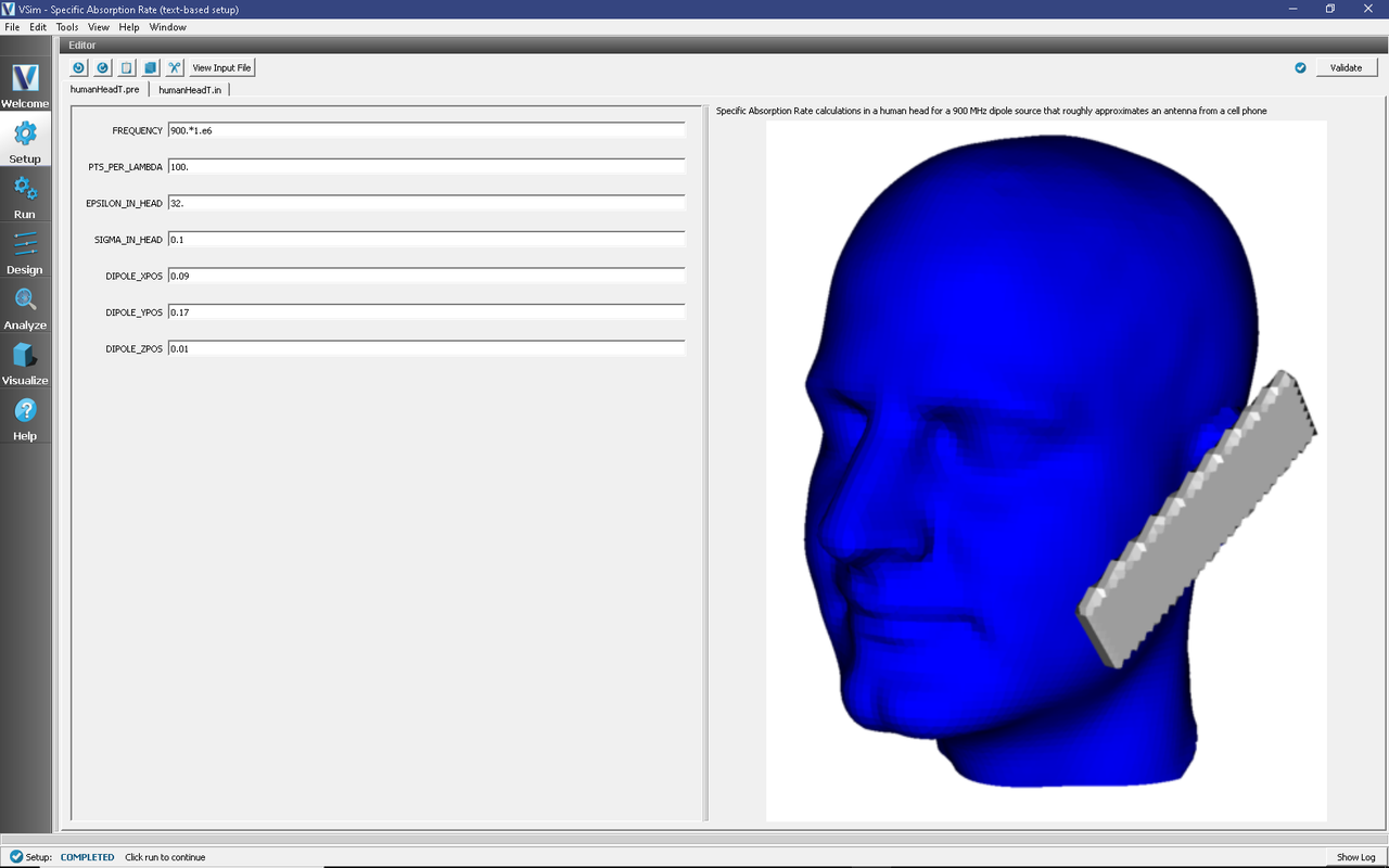
Fig. 330 Setup window for the Human Head example.
Input File Features
The input file allows one to select the frequency of the dipole source as well as the number of grid points to include per wavelength for the wave in a vacuum. One can also set the dielectric value and conductivity value in the human head. We have also included the ability to select the position of the dipole source approximating the cell phone antenna. A voxel representation of the human head can also be used for more specific tissue values via a voxel dat file with python.
Running the Simulation
After performing the above actions, continue as follows:
Proceed to the run window by pressing the Run button in the left column of buttons.
To run the file, click on the Run button in the upper left corner of the right panel. You will see the output of the run in the right pane. The run has completed when you see the output, “Engine completed successfully.” This is shown in Fig. 331.
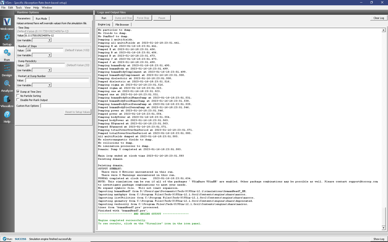
Fig. 331 The Run window at the end of execution.
Visualizing the Results
After performing the above actions, continue as follows:
Proceed to the Visualize window by pressing the Visualize button in the left column of buttons.
To create the image shown in Fig. 332:
Expand Scalar Data
Select E and ESquared
Select Log Scale Color
Select Display Contours and set the # of contours to 7
Select Clip Plot and in the Plane Controls set the Clip Plane Normal to X and set the Origin Of Normal Vector to X = 0.1, Y = 0, Z = 0
Expand Geometries
Select poly
Move the dump slider forward in time
Click and drag with the mouse to rotate the image
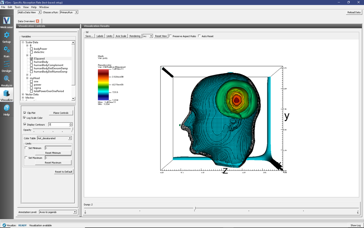
Fig. 332 Visualization of the absorption of power by a human head via a clip.
Further Experiments
We suggest the user change the frequency of the dipole source to imitate different cell phone models at different frequencies.
We also suggest the user change the position of the dipole implying a change in location of the cell phone antenna.
It would also be interesting to change the dielectric and conductivity value to model a dipole source in a vacuum.