Multimode Fiber Mode Extraction (multiModeFiberModeExtract.sdf)
Keywords:
- Photonics, dielectric fiber
Problem Description
This example illustrates how to compute the modes of a cylindrical fiber for a given propagation constant, \(\beta\), which, because the primary direction of propagation in VSim is along the \(x-axis\), is also denoted as \(k_x\). The calculation is performed using excitation of a system with only two cells in the \(x-dimension\). (The simulation can be performed with one cell in \(x\), but this cannot be easily visualized so two are used instead.) This document will show how to extract the modes and their frequencies, as well as how to get a text-based setup file for further exploration, including solving for the propagation constant as a function of the frequency.
This simulation can be performed with a VSimEM license.
Opening the Simulation
The Multimode Fiber Mode Extraction example is accessed from within VSimComposer by the following actions:
Select the New → From Example… menu item in the File menu.
In the resulting Examples window expand the VSim for Electromagnetics option.
Expand the Photonics option.
Select Multimode Fiber Mode Extraction and press the Choose button.
In the resulting dialog, create a New Folder if desired, and press the Save button to create a copy of this example.
All of the properties and values that create the simulation are now available in the Setup Window as shown in Fig. 258. Expanding the Constants section of the Simulation Tree shows the user-defined constants of this simulation:
LENGTH_UNIT(real):The length-scale of the simulation. All lengths, such as that of the fiber radius and box size, are divided by this number to make the geometry lengths of order unity as needed by the geometry engine. In this case,
LENGTH_UNITis unity, so it has no effect.WAVELENGTH_VAC(real):Wavelength of the signal in vacuum. Determines the excitation frequency.
N_EFF(real):Estimate of the value of \(n_{eff}\) of the expected modes. This determines the wavenumber, \(k_x = 2 \pi n_{eff}/\lambda_{vac}\), of the modes to be found.
RESOLUTION(real):The resolution of the simulation grid. The cell size is set to be this number multiplied by the smallest simulation feature, i.e., the fiber radius.
XCELLS(integer):The number of cells to simulate in the x direction.
CFL_NUMBER(real):This times the stable time step gives the time step chosen for the simulation.
FREQ_GAP_REL(real):The gap outside of which the excitation drops off to the suppression level. simulation.
Expanding the Parameters section of the tree shows how the other
simulation parameters are computed from the constants. For
example, the grid size DX along the \(x-axis\) is set
to the resolution multiplied by the vacuum wavelength, divided by
\(n_{eff}\) and scaled by LENGTH_UNIT. The
excitation central frequency, frequency, is computed from
the vacuum wavelength scaled by the LENGTH_UNIT. The
longitudinal wavenumber, KAY, is computed from the
desired \(n_{eff}\), and from that the phase shift across
cells along the \(x-axis\) is calculated.
The range of frequencies to be excited is [FREQ_LOW,
FREQ_HIGH ]. Outside of this range by FREQ_GAP,
the excitation drops off to the suppression value. This requires
a successively longer excitation time, TIME_EXCITE and so
a successively larger NSTEPS_EXCITE, the number of
steps for the excitation.
Absorbing layers have been placed at the y and z limits to damp out modes that would be outgoing for a fiber in infinite space.
In 3D View tab of the right pane of the Setup Window, the fiber and the grid are visible. Right-click and drag to rotate the view. The simulation has been constructed so that the fiber extends beyond the grid in both the positive and negative \(x-directions\), with a fiber diameter one-half the perpendicular domain length.
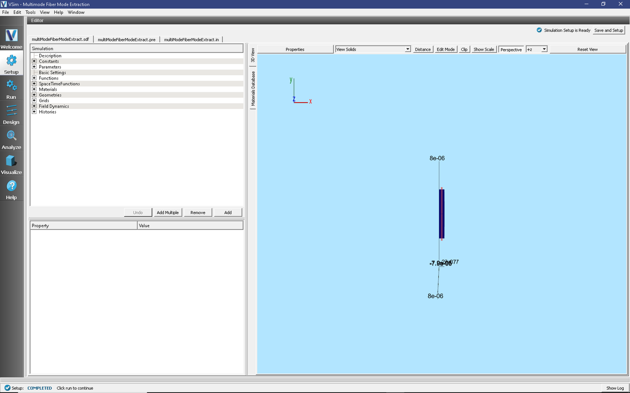
Fig. 258 Setup Window for the Multimode Fiber Mode Extraction example.
Expanding the Materials section of the Simulation tree shows that
the simulation includes FiberMaterial. This was created
by importing a material from the Database tab of the right pane
of the Setup Window, then changing the name of the material and
changing its properties. A material can be changed arbitrarily
once it is in the simulation, as shown in
Fig. 259.
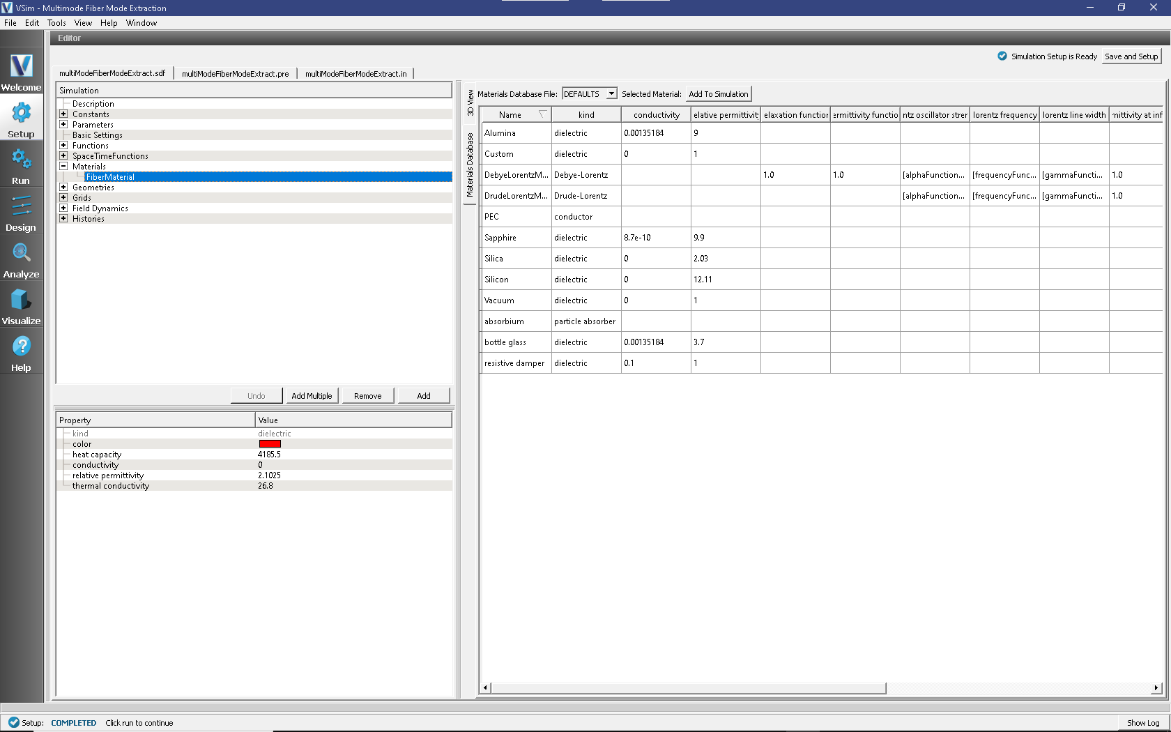
Fig. 259 Setup Window for the Multimode Fiber Mode Extraction materials.
Expanding the Geometries of the Elements Tree shows that the
simulation includes one geometry, the fiber, and its material is
FiberMaterial. This is seen in
Fig. 260.
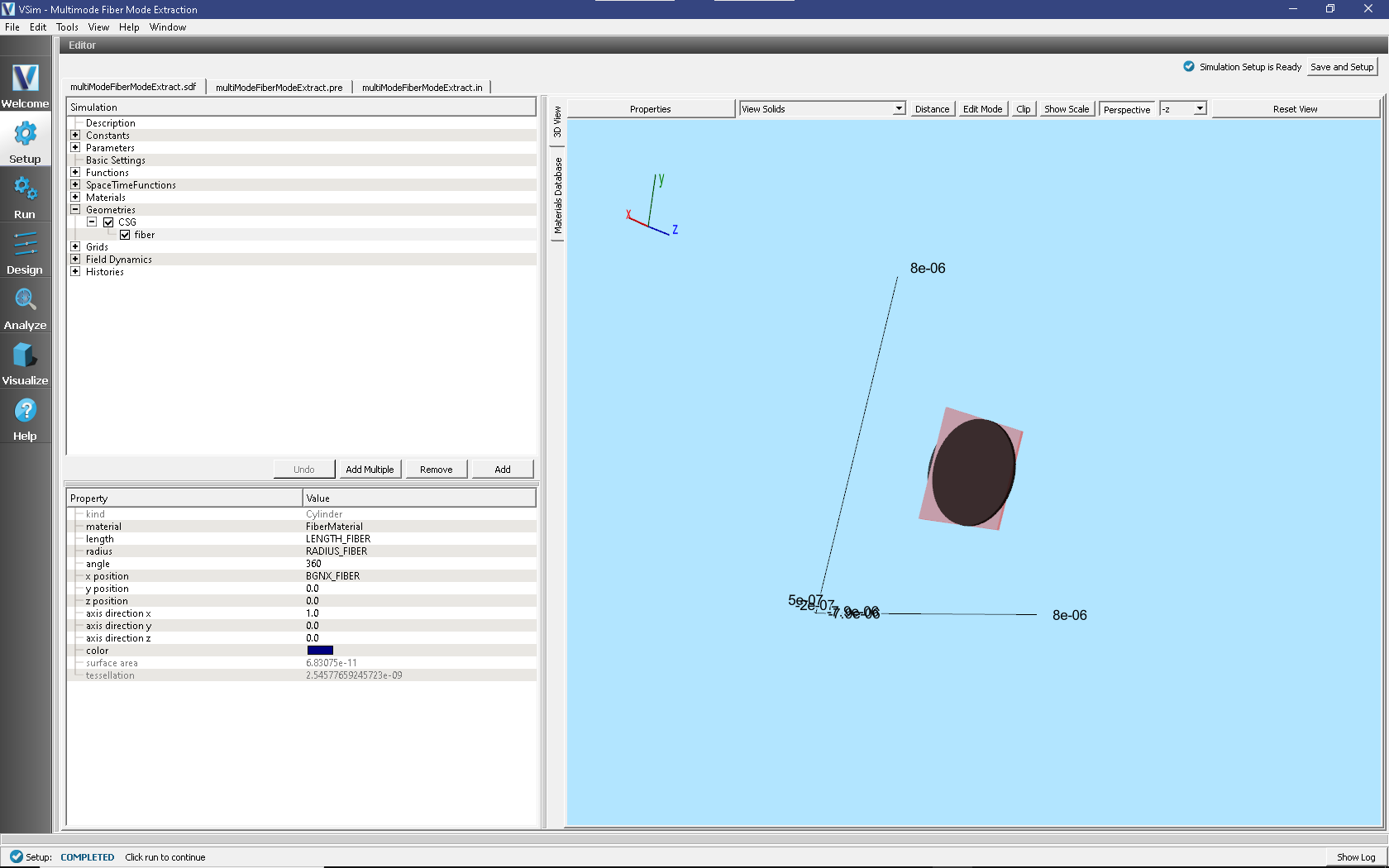
Fig. 260 Setup Window for the Multimode Fiber Mode Extraction geometries.
This simulation is excited with the freqBand function.
This is a function that has a fairly uniform excitation over a
band of frequencies, falling off steeply outside of the band.
The band has been chosen to be centered near where we expect to
find the modes.
A field history has also been implemented in this simulation, so that the Fourier transform of what has been excited can be seen.
As noted above, under the Parameters section of the Tree Elements
is defined NSTEPS_EXCITE which specifies the number of
steps to excite the desired frequency content. Because
FREQ_GAP also distinguishes the peaks, this excitation
time will distinguish the peaks.
Running the Simulation
Once finished with the problem setup, continue as follows:
Proceed to the Run Window by pressing the Run button in the left column of buttons.
For this run we choose 10000 steps, much greater than that (4000) required for the excitation. This further reduces any effect of the excitation on the signal in free oscillation.
Choose parallel computing options on the MPI tab.
To run the file, click on the Run button in the upper left corner of the Logs and Output Files pane. You will see the output of the run in that pane. The run has completed when you see the output, “Engine completed successfully.” This is shown in Fig. 261.
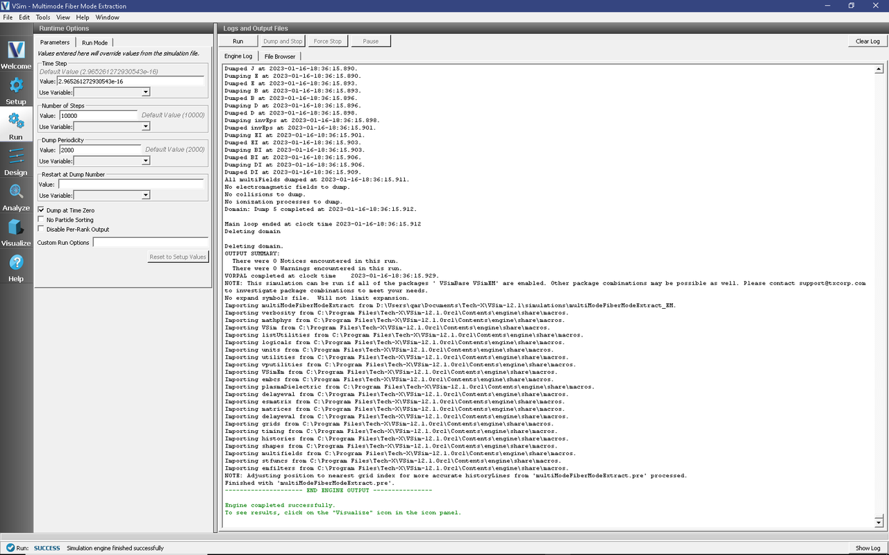
Fig. 261 The Run Window at the end of execution.
This simulation takes approximately 10 seconds on 4 cores of a modern processor.
Visualizing the spectrum
Proceed to the Visualize Window by pressing the Visualize button in the left column of buttons.
In the Visualization Controls pane, in the dropdown menu for Add a Data View select History.
For graph 1, set the quantity to be plotted to
driveCurrent_2.For graph 2, set the quantity to be plotted to
midUpperRightE_2.In the Visualization Results pane, for each plot, click the Fourier Amplitudes (dB) check box.
Graph 1 shows the square window in frequency space.
Graph 2 shows several peaks between 200 and 250 THz.
To see this region in more detail, for each graph press the limits button and set the minimum to 1.7e14 and the maximum to 2.7e14. Peaks in the spectrum are seen at the frequencies, 198 THz, 205THz, 217THz, 233, and several around 250 THz in Fig. 262.
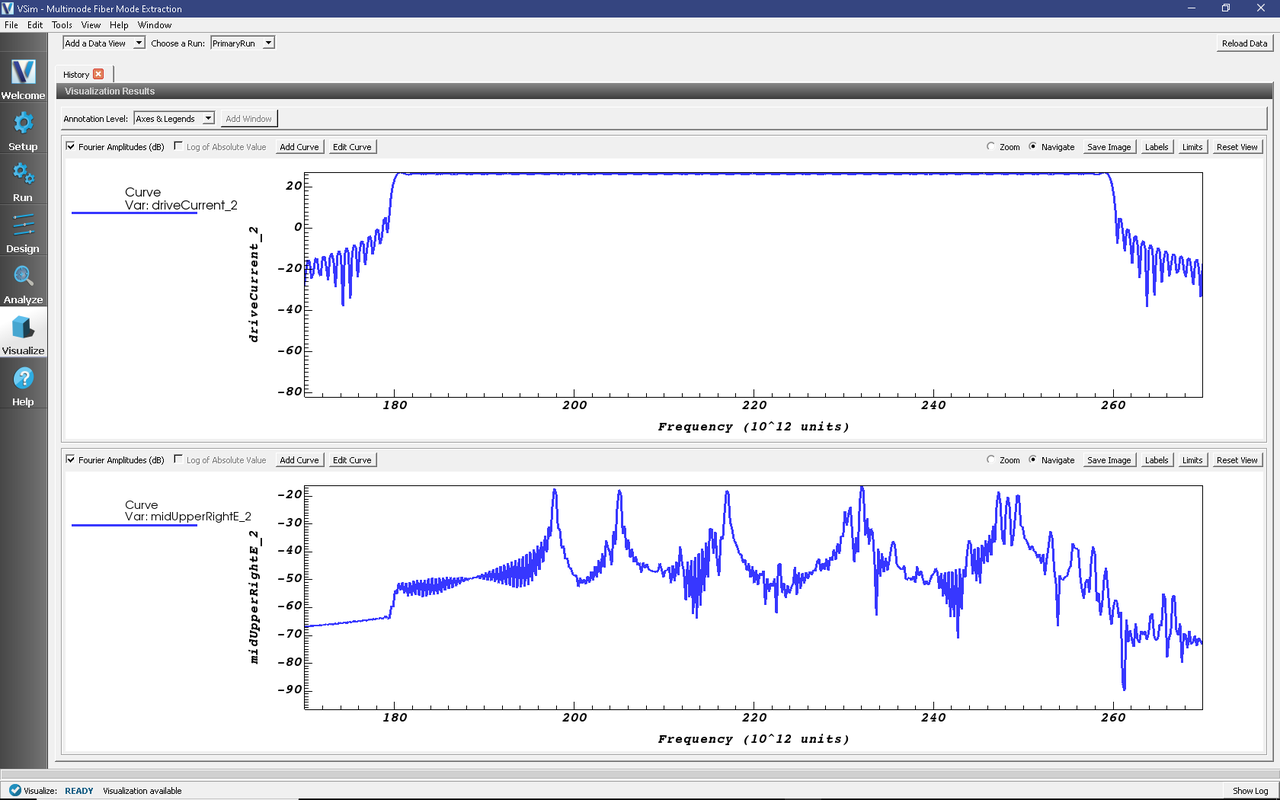
Fig. 262 The observed spectrum.
Analyzing the Results
Since 8 modes were seen, we look for 8. This will require 3 dumps per mode, or about 24 additional dumps. The dumps should be spread out over a few oscillations (35 steps each) or so, and it is good to do a few extra. To get these new dumps, return to the Run pane, set Number of Steps to 200, Dump Periodicity to 5, and Restart at Dump Number to 5. This will start a new simulation from where the first stopped. Click the Run button in the top left corner of the right pane.
Now go to the Analyze pane, select the extractModes.py analyzer, and press the Open button. Set the field to E, choose beginDump to be 6, endDump to be 45, nModes to be 8, and 100 of each kind of points. Also check the boxes next to randomSample and construct. Upon hitting the Analyze button of the Analyze pane, we sees the list of detected frequencies, of which the first (mode 0) is the mode of interest, it having frequency of 1.98e14. This is seen in Fig. 263.
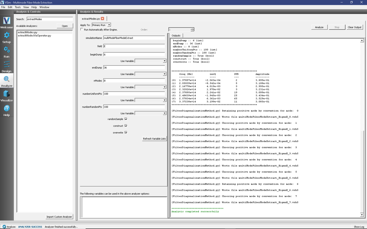
Fig. 263 Extraction of the mode frequencies.
Note
The sign of the mode may vary on different operating systems. So, the visualization of the Eigen modes could be different from what is seen in Fig. 263.
Visualizing the eigenmodes
Return to the Visualize Window, reload the data, open Scalar Data -> E, and click on E_z (EigenE). Keep the slider on position 0. With the mouse, turn the image sideways to see the cross section, as shown in Fig. 264.

Fig. 264 The extracted eigenmode.
Convergence
This simulation can be repeated for different values of
RESOLUTION to see how the frequency varies with the
meshing. We carried out this experiment with RESOLUTION
varying over 0.1, 0.05, 0.02, 0.01 and plotted the frequency
versus the inverse grid length in
Fig. 265.
For each value of the resolution do the excitation run followed by the extraction run:
Excitation run: Press Reset to Setup Values to get the correct value for the time step. Then set the number of step in the run panel to what is given by
NSTEPS_EXCITE, and also modify the number of steps in the second run proportionately. E.g., forRESOLUTION= 0.05,NSTEPS_EXCITE= 7916, so in the Run panel choose Number of Steps = 8000 and Dump Periodicity = 2000. Clear the Restart at Dump Number box. Press the Run button.Extraction run: E.g., for
RESOLUTION= 0.05, set the Number of Steps to 400, the Dump Periodicity to 10, and Restart at Dump Number to be 4.Analysis: Same as originally, as all numbers have been scaled.
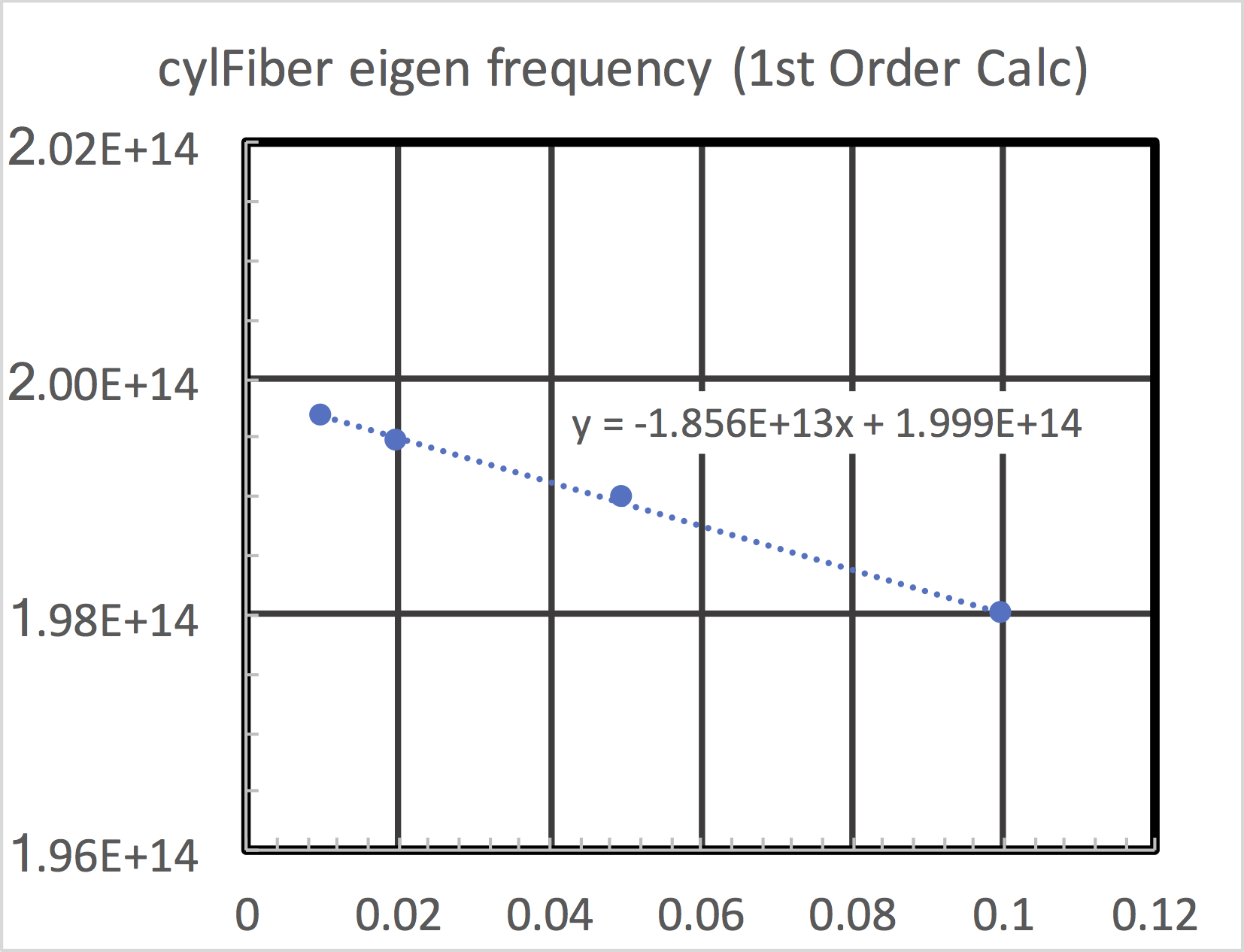
Fig. 265 Convergence of the first mode.
The linear approach to the axis indicates that this is a first order accurate calculation. In other examples we will show higher-order accuracy. Even so, one can see that the frequency is obtained on the sub-percent level with the finest grid used.
Further Experiments
This same process can be used to get the frequency of modes of different wavelengths or of waveguides of different cross sections or made of different dielectrics.