Ionization Injection (fieldIonizeT.pre)
Keywords:
- laser plasma accelerator, controlled injection,
- ionization of high-Z gas
Problem description
This example demonstrates the use of VSim to simulate ionization-induced injection in a laser plasma accelerator [CES+12]. An intense laser pulse propagates up a plasma density ramp into a uniform plasma, which creates a wakefield. Neutral nitrogen atoms are added to the pre-ionized gas at the beginning of the plasma, where the laser pulse field ionizes them. If the electrons released from the nitrogen ionization are at the correct position relative to the wakefield phase, they can be trapped and accelerated to high energy [CCMG+13].
The laser envelope has a Gaussian profile defined at the waist position by (X_0_LASER):
\[E_z = E_0 \exp\left(-x^2/LPUMP^2\right)\exp\left(-(y^2+z^2)/W\_0^2\right) \sin \left( \omega_0 t \right)\]
where \(\omega_0=2\pi c\ /\) WAVELENGTH is the laser
frequency. The laser amplitude is defined through the normalized
vector potential A_0 = \(eE_0/ \omega_0 m_e c\).
This simulation can be performed with a VSimPA license.
Opening the Simulation
The Ionization Injection example is accessed from within VSimComposer by the following actions:
Select the New → From Example… menu item in the File menu.
In the resulting Examples window expand the VSim for Plasma Acceleration option.
Expand the Laser Driven Acceleration (text-based setup) option.
Select “Ionization injection (text-based setup)” and press the Choose button.
In the resulting dialog, create a New Folder if desired, and press the Save button to create a copy of this example.
The basic variables of this problem should now be alterable via the text boxes in the left pane of the Setup Window, as shown in Fig. 495.
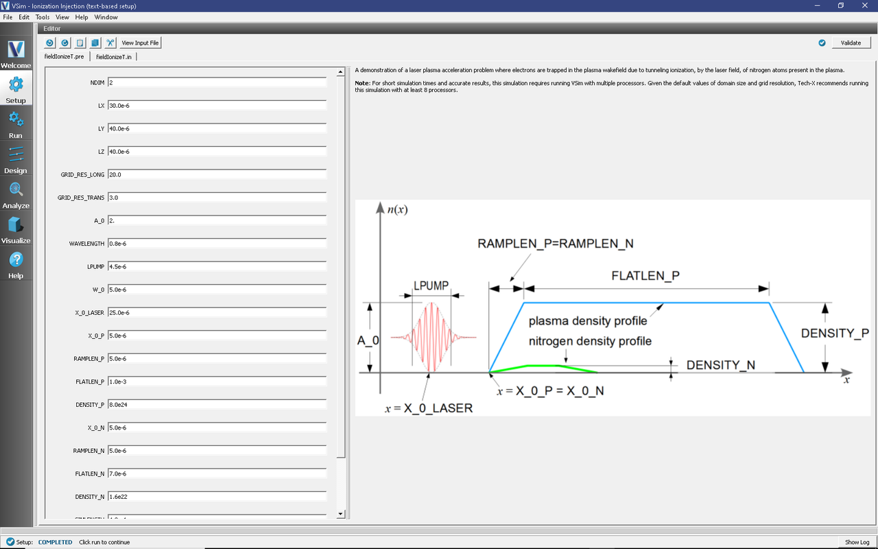
Fig. 495 Setup Window for the Ionization injection in Laser Plasma Accelerator example.
Input File Features
The simulation setup consists of an electromagnetic solver using the Yee algorithm. The laser pulse is launched from the left side of the window using an expression launcher at the boundary. MALs are used on the transverse sides of the window to absorb outgoing waves. The plasma is represented by macro-particles which are moved using the Boris push. The particles are variably weighted to represent the density ramp. The nitrogen atoms are represented using a fluid neutral gas. The different excited levels of the nitrogen and electrons product of the ionization are represented through variably weighted macro-particles. The ionization process takes place in MonteCarlo interactions, using the modified time-resolved ADK formula [CES+12].
Running the Simulations
After performing the above actions, continue as follows:
Proceed to the Run Window by pressing the Run button in the left column of buttons.
This run is computationally intensive, so you click Run in Parallel and select a number of cores equal to the number of physical cores on your machine.
To see the initial evolution, set the Number of Steps to 1000 and the Dump Periodicity to 500.
To run the file, click on the Run button in the upper left corner of the Logs and Output Files pane on the right. of the window. You will see the output of the run in that same pane. The run has completed when you see the output, “Engine completed successfully.” This is shown in Fig. 496.
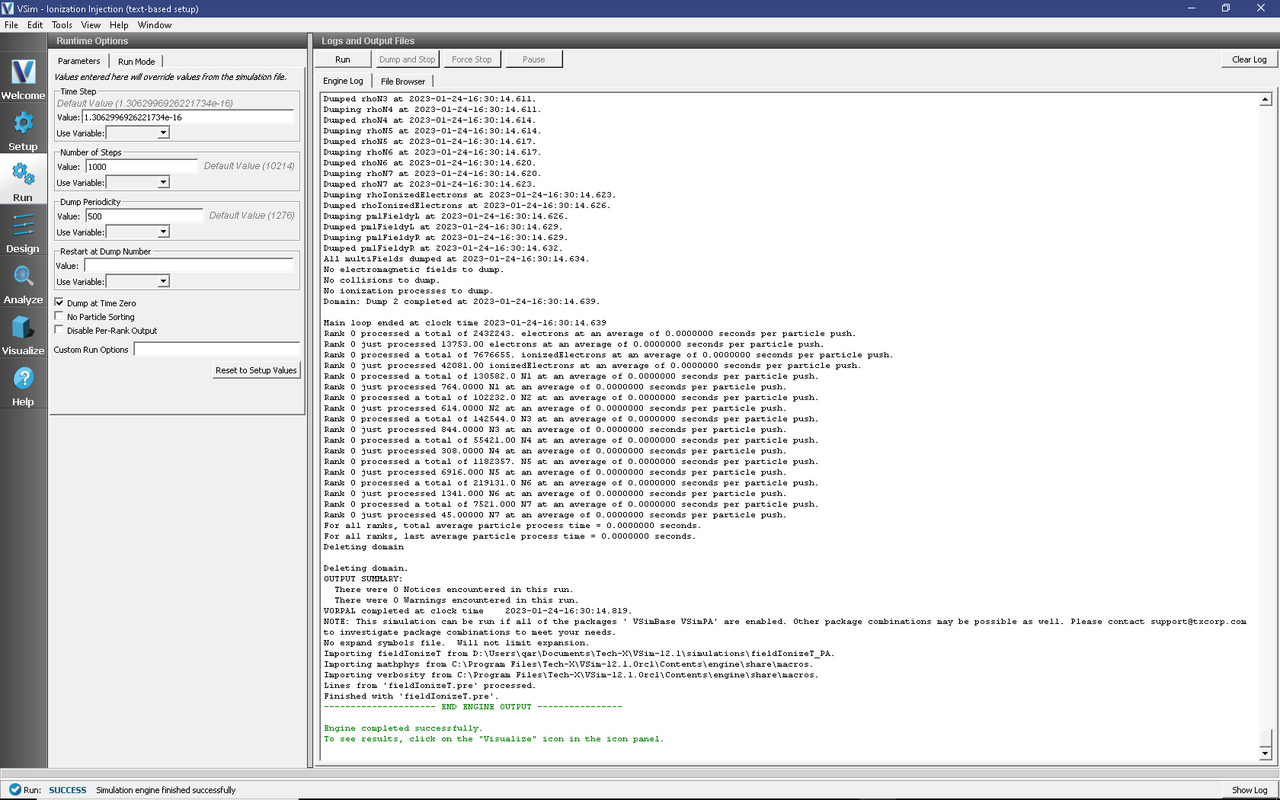
Fig. 496 The Run Window at the end of the first execution.
At this point, one can skip ahead to the visualization section to see whether the fields look reasonable. If they do, you can restart:
Set the Number of Steps to 9000 and Restart at Dump Number to 2.
Click on the Run button. The run has completed when you see the output, “Engine completed successfully.”
This run takes about 70 minutes on a 4 core, 2.5 GHz Intel I7. To run on less powerful hardware one can reduce the number of grid points and number of particles per cell, however physical results may not be as accurate.
Visualizing the Results
After performing the above actions, continue as follows:
Proceed to the Visualize window by pressing the Visualize Tab in the left column of buttons.
The laser pulse is the \(z\) component of the field, while the accelerating
field is the \(x\) component. The plasma density can be seen
in rho.
Fig. 497 shows the longitudinal laser field along the beam axis. To reproduce:
Set Data View to Field Analysis
Select edgeE_x from the Field drop down menu
Select the Horizontal tab in the lineout settings
Set the intercept to
0Click “Perform Lineout
Click Auto Reset on both the pseudocolor and lineout plots so that the window updates the plot region as one moves the slider. You may need to expand your visualization window for the Auto Reset checkbox to appear.
Move the dump slider forward in time
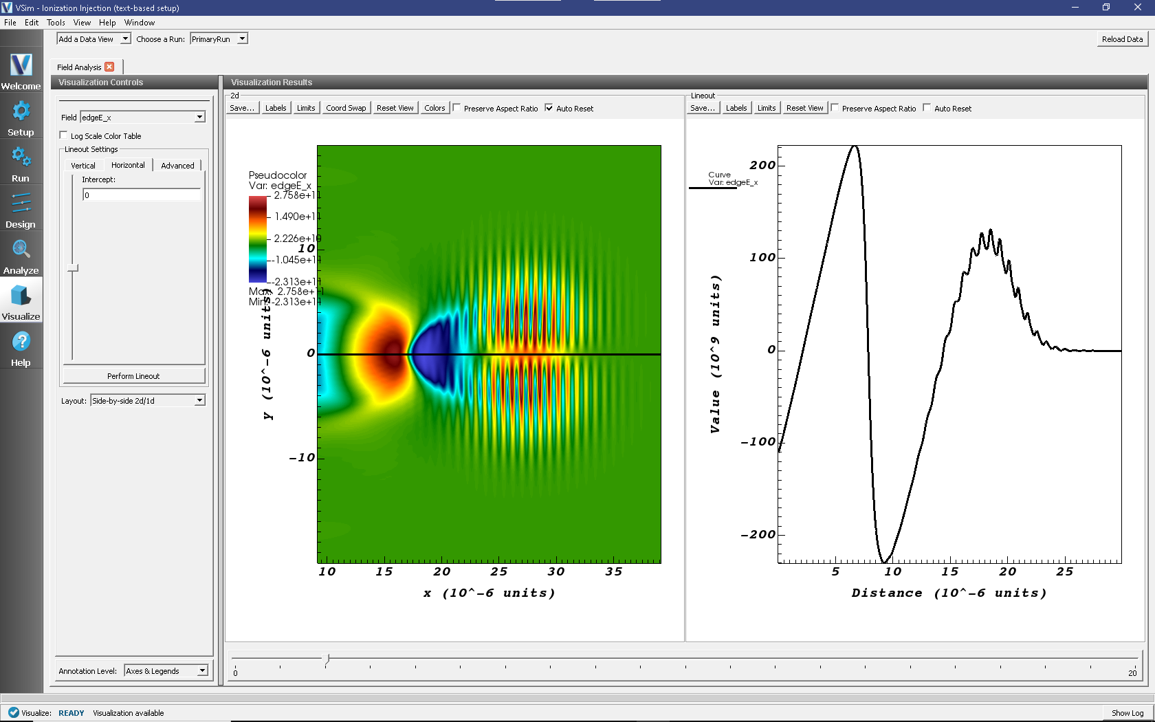
Fig. 497 Left: Longitudinal electric field \(E\)x\((x,y)\) at t=1.3 picoseconds. Right: Line-out of field plot at \(y\) = 0.
The acceleration of the particles can be seen by viewing the (\(x\)) component of the velocity as shown in Fig. 498
Set Data View to Phase Space
Set Base Variable to electrons
Set the X-axis variable to electrons_x, the Y-axis variable to electrons_ux
Check Enable Second Plot
Set Base Variable to ionzedElectrons
Set the X-axis variable to ionizedElectrons_x, the Y-axis variable to ionizedElectrons_ux
Click Draw
Click Reset View or Click Auto Reset on the plot so that the window updates the plot region as one moves the slider. You may need to expand your visualization window for the Auto Reset checkbox to appear.
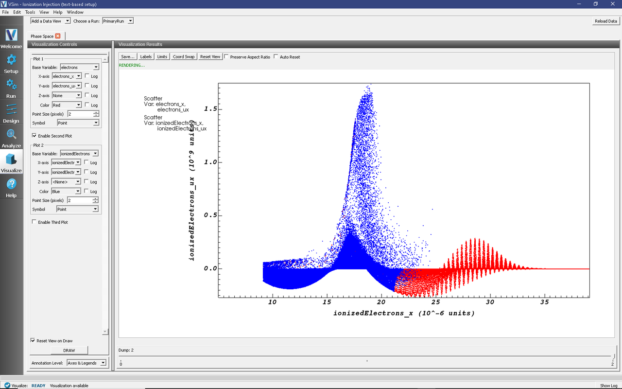
Fig. 498 Phase-space plot (\(x\), \(\gamma\ v\)x) of plasma electrons at t=0.33 picoseconds.