1D Capacitive Plasma Chamber (capacitivelyCoupledPlasma1D.sdf)
Keywords:
- CCP discharge, secondary emission, elastic collision, excitation, ionization.
Problem description
The capacitively coupled plasma (CCP) is one of the most common types of industrial plasma sources. The discharges usually take place between metal electrodes in a reaction chamber and are driven by a radio-frequency (RF) or DC power supply. The plasma is sustained by ohmic heating in the main body and stochastic heating through a capacitive sheath.
This example demonstrates the generation of a capacitively coupled plasma inside two parallel conducting plates separated by 0.05 m. A background Ar neutral gas at approximately 6 mTorr (a number density of approximately \(2.0 \times 10^{20} \ m^{-3}\)) is filled between the electrodes. The right electrode is grounded, while the left one is connected to a voltage source of 200 V at 60 MHz.
This simulation can be performed with a VSimPD license.
Opening the Simulation
The 1D Capacitively Coupled Plasma Discharge example is accessed from within VSimComposer by the following actions:
Select the New → From Example… menu item in the File menu.
In the resulting Examples window expand the VSim for Plasma Discharges option.
Expand the Capacitively Coupled Plasmas option.
Select “1D Capacitive Plasma Chamber” and press the Choose button.
In the resulting dialog, create a New Folder if desired, and press the Save button to create a copy of this example.
The Setup Window and elements tree with all the implemented physics and geometries, is shown in Fig. 490.
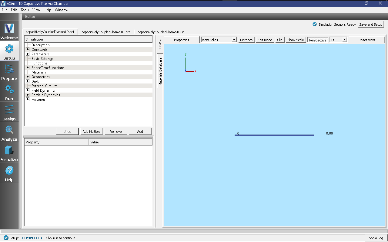
Fig. 490 Setup Window for the 1D Capacitively Coupled Plasma Discharge example.
The time step DT should sufficiently resolve the plasma frequency and collision frequency. The default time step used in this example is (TIMESTEP_FACTOR * 0.1) / PLASMA_FREQUENCY to ensure stability. The initial primary electrons are gradually loaded into the simulation domain over a period of LOADSTEPS timesteps, which has a default value of 5000.
Simulation Properties
This simulation includes some constants and parameters for easy adjustment of the simulation properties. These include:
Constants
NEUTRAL_ARGON_DENSITY: number density of the background neutral argon gas (number/m^3).
FREQUENCY: sets the frequency of the driving voltage set on the lower X boundary.
VOLTAGE: sets the amplitude of the driving voltage set on the lower X boundary.
NOMINAL_DENSITY: this adjusts the number of physical particles loaded into the simulation.
LOADSTEPS: Timestep when particle loading will end.
NSTEPS: How many timesteps to simulate.
STEPS_PER_DUMP: number of steps to take between data dumps.
BMAG: sets the strength of the magnetic field (default = 0T).
Time-dependent Dirichlet boundary conditions are used to set up the boundaries of electric fields around the reaction chamber walls, and are set in Field Dynamics -> FieldBoundaryConditions. The self-consistent electric field is solved from Poisson’s equation by the Generalized Minimum Residual (gmres) electrostatic solver in Cartesian coordinates. For more information on the solver, see the Reference Manual. This solver is chosen under Field Dynamics -> PoissonSolver.
The plasma is represented by macroparticles which are moved using the Boris pusher in Cartesian coordinates and interact with the background neutral argon gas through collisions set up with the Reactions framework. The particles, background gas, and collisions are set up in the Particle Dynamics Element.
The simulation includes two electron species: Primary electrons which are electrons loaded into the simulation, and Secondary electrons which are created through physical processes. Both species are managed weight particle species, which will combine or split macro particles based on user choices. See the Charged Particles section of the Reference Manual for further information on managed weight particles.
Elastic collisions between electrons and the background gas, excitation collisions in which an electron will lose energy to the background gas, and ionization collision in which electrons create argon ions from the background gas are all included. The cross-sections for this collisions are imported from 2-column data files.
Running the simulation (NOTE: Need to remake capacitivelyCoupledPlasma1DRunWin.png: run window has changed)
After performing the above actions, continue as follows:
Proceed to the Run Window by pressing the Run button in the left column of buttons.
To run the file, click on the Run button in the upper left corner of the Logs and Output Files pane. You will see the output of the run in this pane. The run has completed when you see the output, “Engine completed successfully.” This is shown in Fig. 491.

Fig. 491 The Run Window at the end of execution.
Visualizing the results (NOTE: History plot needs to be re-done since history format has changed starting in VSim 12)
After performing the above actions, continue as follows:
Proceed to the Visualize Window by pressing the Visualize button in the left column of buttons.
From the “Data View” option, select “History”. There are 6 histories that can be plotted in this window: the number of physical particles and the number of macro particles for each of the three particle species (argon ions, primary electrons, and secondary electrons). To produce the plot in Fig. 492 follow these steps:
Plot the ‘numArgon’ history in Graph 1.
Plot the ‘numPrimaryElec’ history in Graph 2.
Plot the ‘numArgon’ history in Graph 3 and change the Location to Window 2
Plot the ‘numPhysSecondaryElec” history in Graph 4.
The simulation converges as the number of secondary electrons approaches a constant, indicating a steady state plasma. With the default number of time steps (4000, or 20 nanoseconds), the simulation does not reach steady state (see the black, numPhysSecondaryElec history curve). To reach steady state, the simulation must run for approximately 100 microseconds.
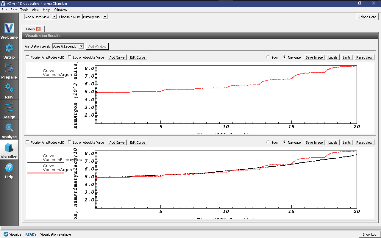
Fig. 492 Visualization of number histories of ion, primary electron, and secondary electrons for 4000 steps or 20 nanoseconds.
Further Experiments
Set up a History that records the electron current flowing into the left and right sides of the simulation. Right click on the “Histories” element in the Setup Window and under “Add ParticleHistory” select “Absorbed Particle Current.” You can change the name of the history by double clicking on the new “absorbedPtclCurrent0” element in the tree. Then be sure to pick the particle absorber from which you would like to collect data.
The Reactions framework allows one to set up collision interactions flexibly. The collisions involved in this example are electron-neutral collisions that lead to ionization and ohmic heating. As a further experiment, ion-neutral collisions, such as elastic scattering and charge exchange, can also be added to the simulation.
The VSim interface can import any cross sections that are in a 2-column format. There should be NO headings in the data file. The LXcat scattering database (https://fr.lxcat.net/data/set_type.php) and EEDL cross section database contain cross section data for around one hundred different materials. As another experiment, change the cross-section used in the simulation or change the species of the background gas and import new cross-sections.