Drifting Electrons (driftingElectrons.sdf)
Keywords:
- electron transport, electron mobility, monte carlo, electrostatic
Problem description
VSim may be used to model charged particles drifting in a background neutral gas. When charged particles, such as electrons, are injected into a background neutral gas, collisions between gas atoms and electrons eventually lead to thermal equilibrium, and electrons will reach the same temperature as the background gas. However, when an external electric field is applied across the neutral gas, the electron collisions and distribution will change due to this applied field. Electrons will gain energy from the applied electric field. The energy loss due to electron-atom collision is small, and most of the energy ends up heating the electrons. Assuming only elastic collisions take place between electrons and atoms, the electron mobility is defined as
\(\mu_{e} = (\frac{\pi\lambda}{2mE})^\frac{1}{2}\)
which describes the relation between electron drifting velocity and applied electric field.
This simulation can be performed with a VSimPD license.
Opening the Simulation
The Electron Drifting example is accessed from within VSimComposer by the following actions:
Select the New → From Example… menu item in the File menu.
In the resulting Examples window expand the VSim for Plasma Discharges option.
Expand the DC Plasmas option.
Select “Drifting Electrons” and press the Choose button.
In the resulting dialog, create a New Folder if desired, and press the Save button to create a copy of this example.
The Setup Window is now shown with all the implemented physics and geometries, if applicable. See Fig. 524.
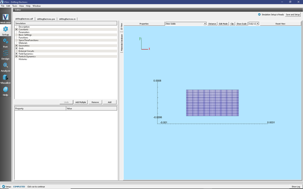
Fig. 524 Setup Window for the Electron Drifting example.
Simulation Properties
This input file contains electron as kinetic species as well as a background fluid description of a gas. Elastic collisions between kinetic particles and the background gas are described by Monte Carlo interaction blocks of kind impactIonization.
The fields are solved for electrostatically at each time step, including the fields due to all charged particles, subject to the boundary conditions specified in the input file. There are a number of histories that record the number of particles for electrons.
Running the Simulation
After performing the above actions, continue as follows:
Proceed to the Run Window by pressing the Run button in the left column of buttons.
To run the file, click on the Run button in the upper left corner of the Logs and Output Files pane. You will see the output of the run in this pane. The run has completed when you see the output, “Engine completed successfully.” This is shown in the window below.

Fig. 525 The Run Window at the end of execution.
Visualizing the Results
After run completion, continue as follows:
Proceed to the Visualize Window by pressing the Visualize button in the left column of buttons.
To view the phase space distribution for the drifting electrons, select Phase Space from the drop down Add a Data View tab. This will open a new tab called Phase Space. In Base Variable, select electrons. Select electrons_x for X-axis and electrons_ux for Y-axis. Click DRAW and move the Dump slider to view electron accelerating and scattering when they drift over the space. The electron phase space at dump number 10 is shown in Fig. 526.
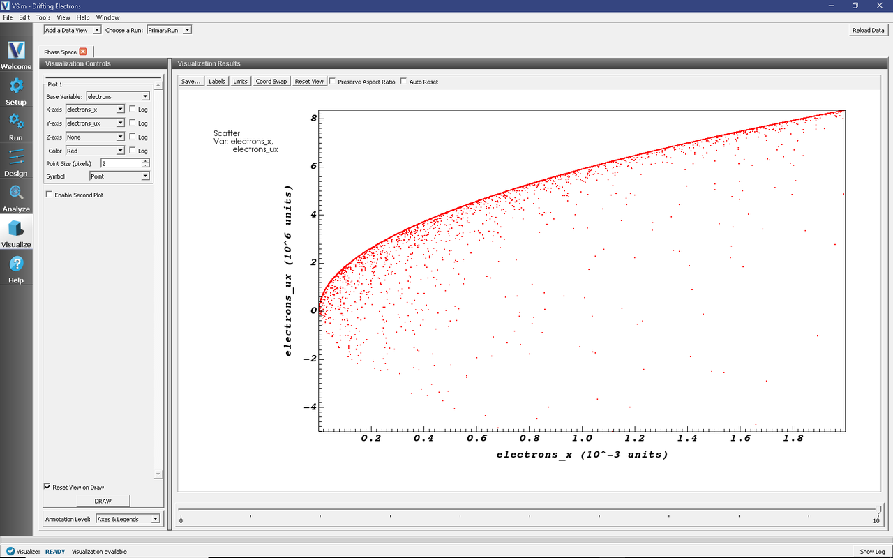
Fig. 526 Electron phase space at Dump 10.
Further Experiments
At lower applied electric fields, electrons are more collisional due to increased cross section. Try reducing the CATHODE_POTENTIAL, and observe more scattered electron distribution when drift over space.
At higher applied electric fields, not only elastic collisions, but also inelastic collisions will take place between electrons and atoms, which further reduce electron drifting velocity and mobility. For further experiments, try adding other collision types, such as excitation and ionization, and observe the effects to electron drifting velocity.