Langmuir Probe (langmuirProbe.sdf)
Keywords:
- electrostatics, particle in cell, sheath, box bounding, internal boundary
Problem description
This example computes the fields and particles in a box, with an interior probe, modeled as a particle absorber and a constant-voltage (Dirichlet) boundary condition. There is an immobile, background neutralizing charge density. The electrons move to the walls and the probe, creating sheaths at all interfaces.
This simulation can be performed with a VSimBase license.
Opening the Simulation
The Langmuir Probe example is accessed from within VSimComposer by the following actions:
Select the New → From Example… menu item in the File menu.
In the resulting Examples window expand the VSim for Plasma Discharges option.
Expand the DC Plasmas option.
Select “Langmuir Probe” and press the Choose button.
In the resulting dialog, create a New Folder if desired, and press the Save button to create a copy of this example.
All of the properties and values that create the simulation are now available in the Setup Window as shown in Fig. 527. You can expand the tree elements and navigate through the various properties, making any changes you desire. The right pane shows a 3D view of the geometry, if any, as well as the grid, if actively shown. To show or hide the grid, expand the Grid element and select or deselect the box next to Grid.
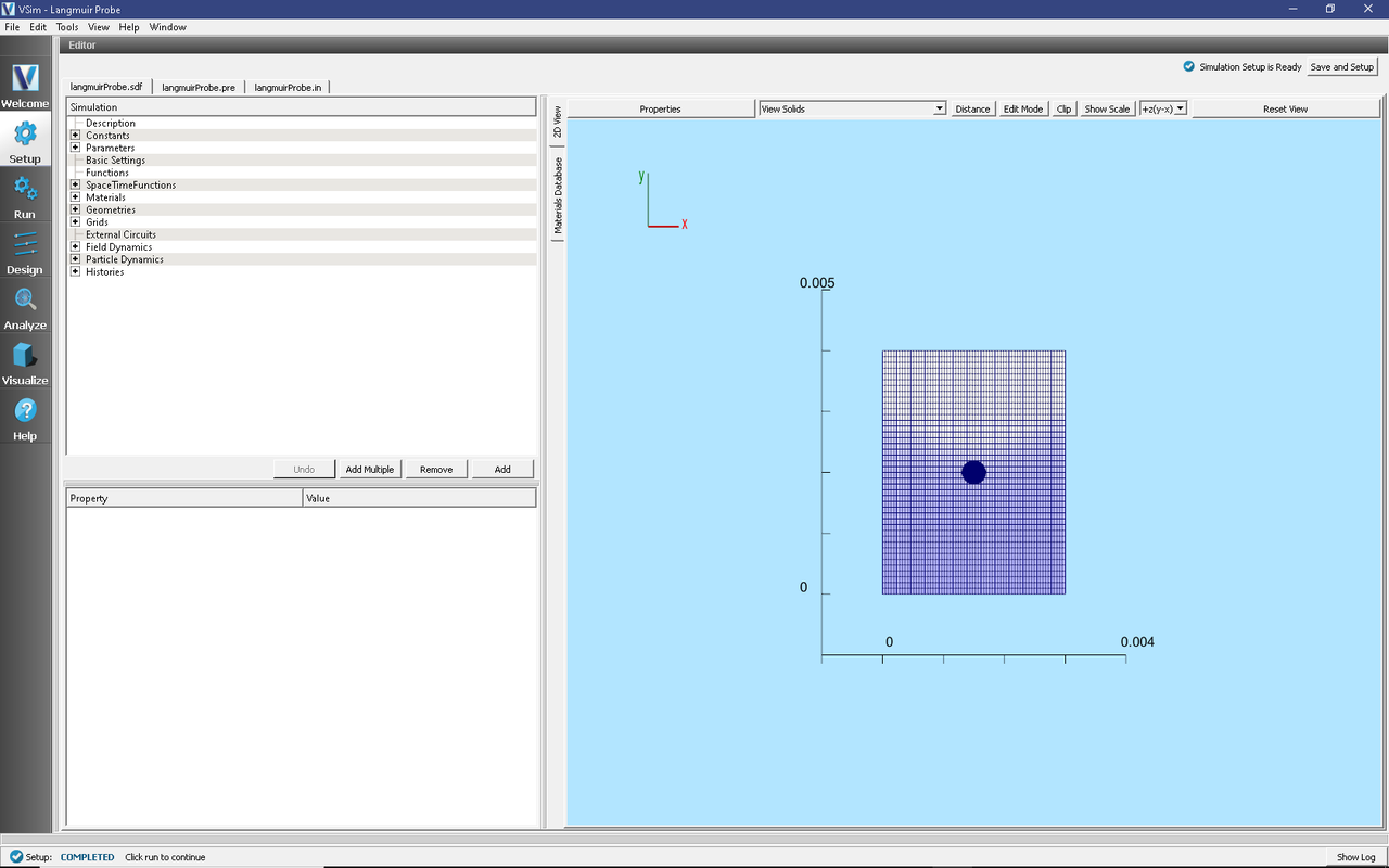
Fig. 527 Setup Window for the Langmuir Probe example.
Simulation Properties
Constants are set up to allow setting the electron temperature in eV (ELEC_TEMP_EV), the electron density (NOM_DENS_E), the number of cells (NCELLS_X, NCELLS_Y) in the x and y directions, the number of particles per cell (PPC), and the size of the simulation (LEN_X, LEN_Y) in the x and y directions.
Running the Simulation
After performing the above actions, continue as follows:
Proceed to the Run Window by pressing the Run button in the left column of buttons.
To run the file, click on the Run button in the upper left corner of the Logs and Output Files pane. You will see the output of the run in this pane. The run has completed when you see the output, “Engine completed successfully.” A snapshot of the simulation run completion is shown in Fig. 528.
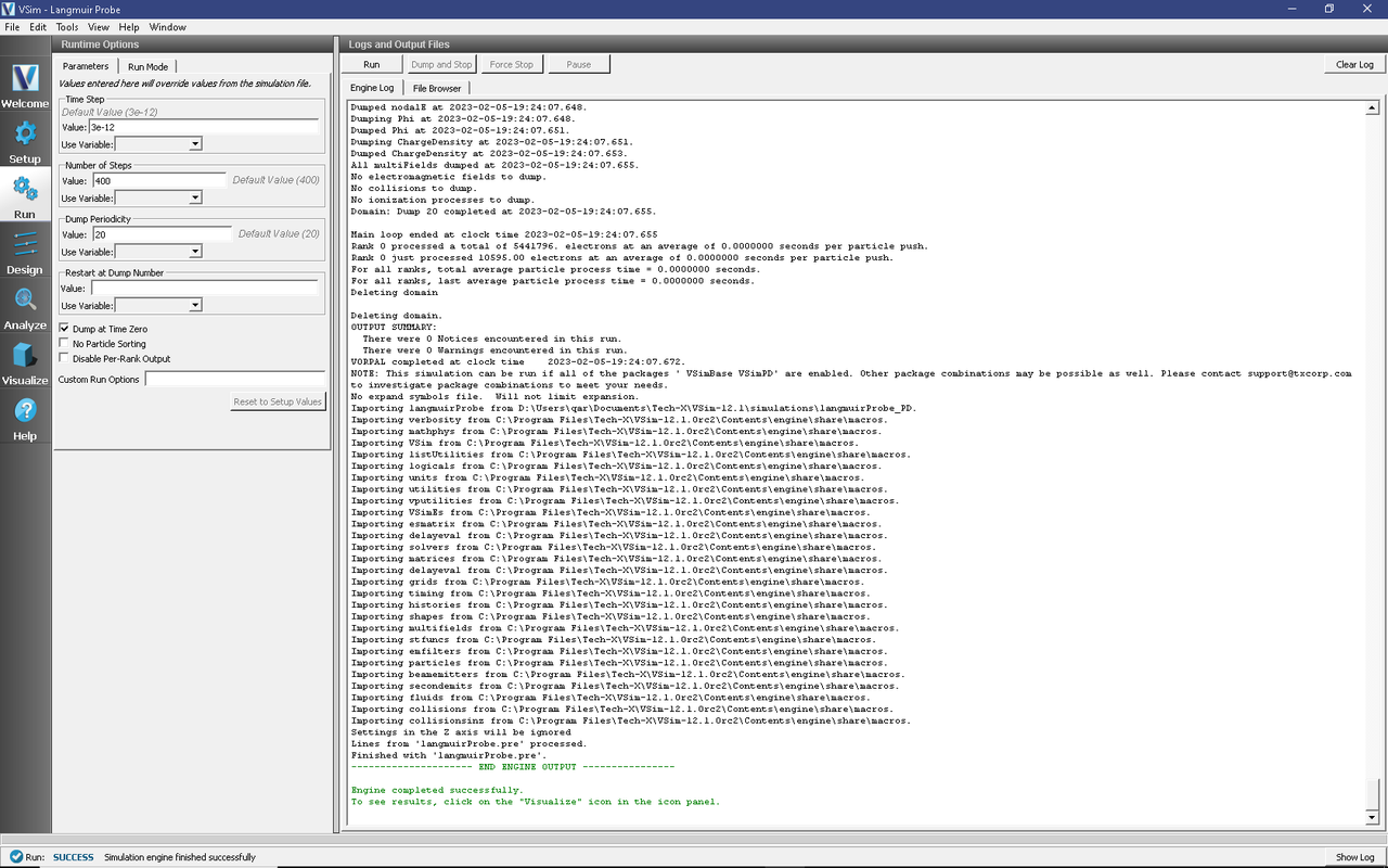
Fig. 528 The Run Window at the end of execution.
Visualizing the Results
After performing the above actions, continue as follows:
Proceed to the Visualize Window by pressing the Visualize button in the left column of buttons.
To view the electric potential, expand Scalar Data in the Data Overview tab and select Phi. The potential in the visualization window resembles that shown in Fig. 529.

Fig. 529 The electrostatic potential
To view the electrons and sheaths, expand the Particle Data, expand electrons and select electrons. Move the dump slider forward in time to see the formation of the sheaths as seen in Fig. 530.

Fig. 530 The sheath formation
Further Experiments
Try adding in another geometry for inclusion of the support rod or try changing the geometry to represent a different probe.