Penning High Intensity Ion Source (PenningSource.sdf)

Keywords:

coherent ion beam, electron emitters, electron-neutral collisions, plasma source

Problem Description

This Penning Source example illustrates how to generate an electron population by emitting electrons off of a cathode using VSim’s Settable Flux Shape Emitter model. The plasma forms due to impact ionization from electron-neutral collisions which ionizes the neutral Argon gas to generate a second electron (in each collision) and a singly charged Argon ion. This simulation also includes impact excitation and elastic collisions between electrons and Argon gas. The various types of elastic and inelastic collisions of the particles are calculated with the Vorpal engine’s Reaction Framework package. The plasma particles, background gas, and collisions are set up in the Particle Dynamics Element. The cross-sections for these collisions are imported from 2-column data files. The electrons are attracted in to the plasma chamber by charging the anode (filled with Argon gas) to a positive potential. Secondary electrons are emitted off the anode due to the primary electrons interacting with the anode walls. This is set up using a Secondary Emitter model in VSim.

The Argon ions are then extracted from the plasma source with two extraction plates biased to a large negative potential. The two extraction plates accelerate the ions out of the plasma generating an ion beam which is focused to a small width according to the space between the two extraction plates. To further focus the ion beam, absorbing plates are placed below the extraction plates which are part of the anode. A 0.16 Tesla magnetic field in the \(y-\textrm{direction}\) is imposed to restrict the motion of the electrons in the Anode region. For the example shown here a Space Time Function is used to confine the magnetic field to a specified region using a Heaviside Step function. The electric field is solved via Poisson’s equation using a Generalized Minimal Residual (GMRES) linear solver. This solver is chosen under Field Dynamics -> PoissonSolver. A combination of Dirichlet and Neumann boundary conditions involving the shapes and simulation boundaries are imposed. Field boundary conditions are imposed under Field Dynamics -> FieldBoundaryConditions. The plasma is represented by macro-particles which are moved using the Boris scheme in a 3D Cartesian coordinate system.

One challange to modeling ion sources using PIC methods is the need to resolve the electron Deybe length to avoid a numerical grid heating instability when the most common PIC methods are used. In this example, the electron density exceeds \(10^{17} \textrm{m}^{-3}\) and the electron temperature is about 3-5 eV. This results in a Debye length that is about \(5 \times 10^{-5}\) m, which would require a grid size \(\approx\) 10 times smaller that what we use in this example (which in 3D would mean the simulation would need a 1000 times more cells than what we use). We avoid this issue by using an energy conserving particle deposition scheme discussed in Reference [1].

This simulation can be run with a VSimPD license.

Opening the Simulation

The Penning Source example is accessed from within VSimComposer by the following actions:

• Select the New → From Example… menu item in the File menu.

• In the resulting Examples window expand the VSim for Plasma Discharges option.

• Expand the Ion Sources option.

• Select Penning High Intensity Ion Source and press the Choose button.

• In the resulting dialog, create a New Folder if desired, then press the Save button to create a copy of this example.

All of the properties and values that create the simulation are now available in the Setup Window as shown in Fig. 553. You can expand the tree elements and navigate through the various properties, making any changes you desire. Please note that many options are available by double clicking on an option and also right clicking on an option. The right pane shows a 3D view of the geometry as well as the grid. To show or hide the grid, expand the “Grid” element and select or deselect the box next to Grid. You can also show or hide the different geometries by expanding the “Geometries” element and selecting or deselecting “anodePlasmaPlate”, “cathode” and/or “extractionPlates”. Note that these three shapes are unions of the other more basic shapes included in this simulation.

Fig. 553 Setup window for the Penning Source example.

Simulation Properties

To demonstrate how to set up the energy conserving particle deposition scheme [1], click on “basic settings” in the elements tree. Under the basic settings option, you will see that the simulation is setup to use an electrostatic field solve, that particles are enabled and that we are invoking the Reactions collisions framework. To create a particle deposition scheme that conserves energy, we have chosen the “particle to field deposition” which we call “smoother energy conserving”. This allows you to run simulation in which the grid size is larger than the electron Debye length and still maintain a physical electron temperature (less than 10 eV). In addition, this example contains many user defined Constants which help simplify the setup and make it easier to modify. The following constants can be modified by left clicking on Setup on the left-most pane in VSim. Then left click on + sign next to Constants and all the constants used in the simulation will be displayed. To add your own constant, right click on Constants and left click on Add User Defined. Below is an explanation of a few of the constants used. There are several more constants included in the simulation.

XSTART/XEND,YSTART/YEND,ZSTART/ZEND: Physical dimensions of simulation in meters.

CATHODE_VOLTAGE: Potential of electron source from which electrons are emitted

ANODE_VOLTAGE: Potential of anode which attracts the electrons from the cathode

PENNING_MAGNETIC_FIELD: Magnetic of external magnetic field used to confine the ion beam

T1: Time that the electrons are emitted from the electron source.

Running the Simulation

Once finished with the setup, continue as follows:

• Proceed to the Run Window by pressing the Run button in the navigation column out left.

• To run the file, click on the Run button in the upper left corner of the Logs and Output Files pane.

You will see the output of the run in that pane. The simulation takes about 1500 time steps before an ion beam is observed to begin forming and 10000 time steps before a persistent modestly dense beam has formed. The run has completed successfully when you see the output, “Engine completed successfully.” This is shown in Fig. 554.

Fig. 554 The Run Window at the end of execution.

Analyzing the Results

After performing the above actions, continue as follows:

• Proceed to the Analysis Window by pressing the Analyze button in the navigation column.

• In the resulting list of Available Analyzers, select computePtclNumDensity.py and press Open

• The analyzer fields should be filled as below:

  • simulationName: penningSource

  • speciesName with “electrons” or “Ar1” which are the names of the two species in the “Particle Dynamics” tab in the visual setup.

• Click Analyze in the top right corner.

• The analysis is completed when you see the output shown in Fig. 555.

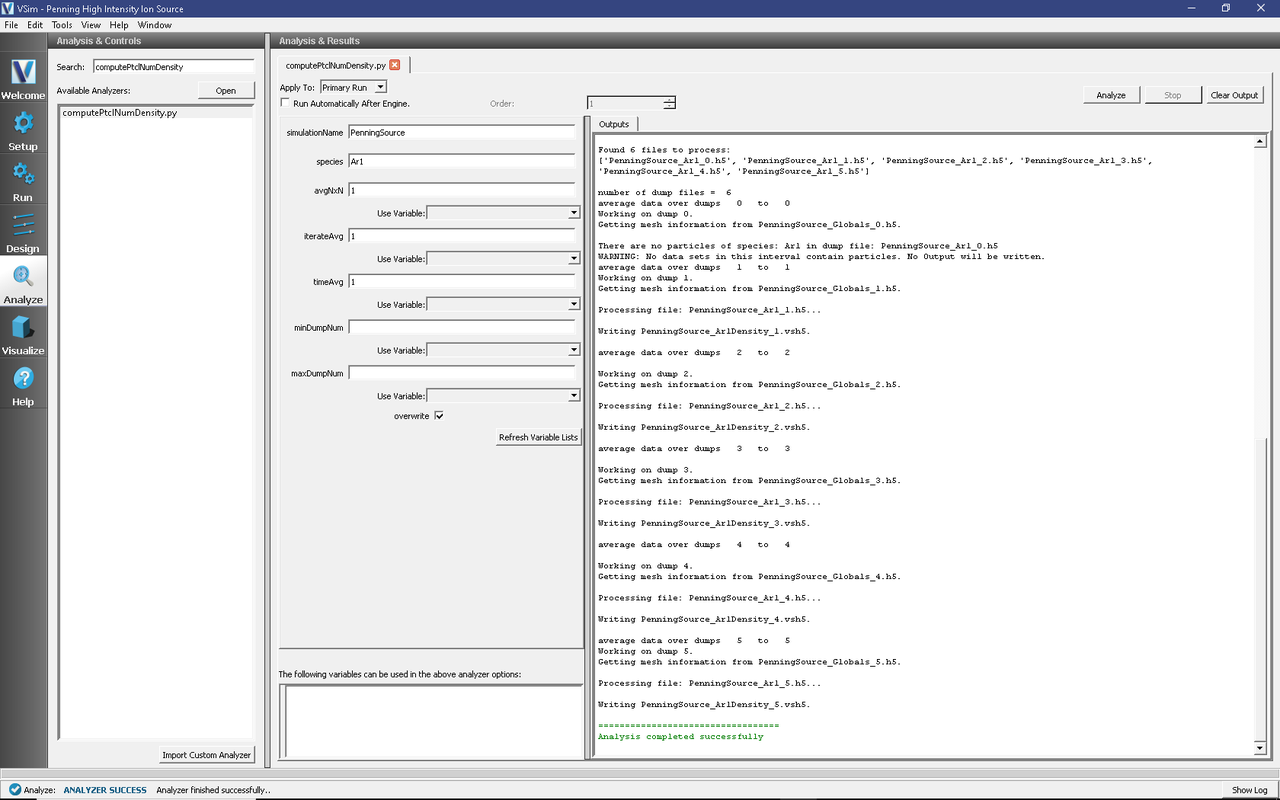
Fig. 555 The Analyze Window at the end of a successful run.

The resulting data is called electronDensity and Ar1Density and shows the number density in the 3D simulation domain in units of #/m^3.

Visualizing the Results

After performing the above actions, the results can be visualized as follows:

• Proceed to the Visualize Window by pressing the Visualize button in the navigation column.

• Clicking on the Add a Data View dropdown menu shows there are many different types of data to visualize.

• To get started, lets visualize the formation of the plasma in the anode and the resulting ion beam.

• Click on the Data Overview tab which is a default tab already loaded in the “Visualize” section of VSim.

• Under Variables, click on “Particle Data”, “electrons” and the top most box (“electrons”)

• Click on “Ar1” then click on the top most box (“Ar1”)

• Finally, to visualize the plasma species in the context of the geometries in the simulation, click on “Geometries”, “poly(cathode)”, “poly(extractionPlates)”, and “poly(anodePlasmaPlate)”.

• You can rotate the figure by holding down the left mouse button and moving the mouse.

• Slide the bar to the right at the bottom of the display window to watch the ions form and accelerate out of the anode.

The resulting visualization is shown in Fig. 556.

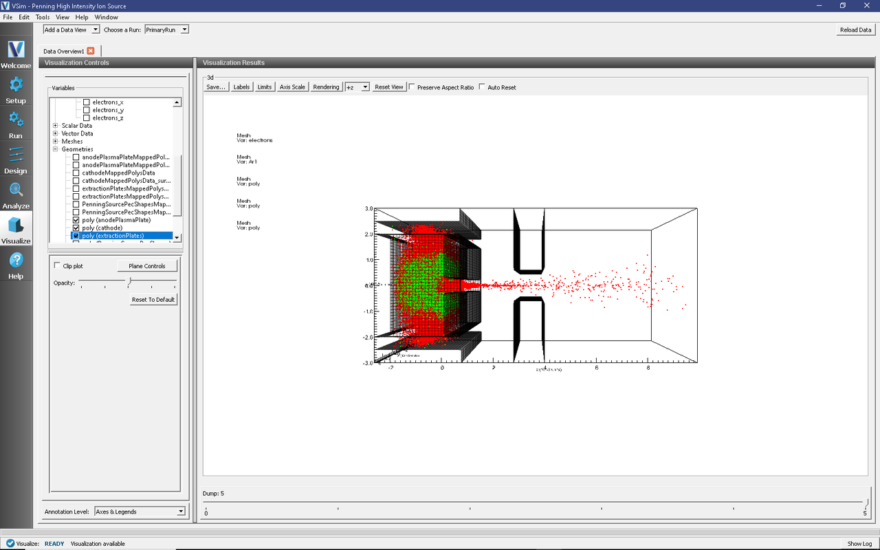
Fig. 556 The evolved ion beam at time step 5000.

This plot shows that the ions have been extracted from the plasma reservoir to form a coherent ion beam.

Next you can visualize the electron density which was generated when you ran computePtclNumDensity.py. To view this dataset, click on “Add a Dataview”, then click on “Field Analysis”. This will open a new plotting window. Click on the region with the “Field” icon, and choose “electronDensity”. You can view this with various configuration. One configuration is to choose “side-by-side 2d/1d” under the “layout” option. This setup is shown in Fig. 557. The option “Preserve Aspect Ratio” is chosen. If you slide the “Lineout Settings” so that a lineout goes through the dense electron region, then you can see that the electron density is \(\approx 10^{16} \textrm{m}^{-3}\).

The visualization window showing phase space is shown in Fig. 557.

Fig. 557 Plot of electron density at time step 5000 in \(\textrm{m}^{-3}\)

Further Experiments

The default example runs for only 5000 time steps. However, the simulation takes 50000 time steps to reach steady state. Therefore, one experiment would be to run the simulation to time step 50000. You should see that the electron density increases to \(\approx 10^{17} \textrm{m}^{-3}\). Since the grid size is \(\approx\) 0.1 mm, the grid size is several times times the electron Debye length. Therefore the energy conserving particle deposition allows for considerable speed up in this calculation.

Set up a History that records the Ar1 current flowing out of the plasma chamber on to the x=XEND boundary. Right click on the “Histories” element and under “Add ParticleHistory” select “Absorbed Particle Current.” You can change the name of the history by double clicking on the new “absorbedPtclCurrent0” element in the tree. Then be sure to pick the particle absorber from which you would like to collect data. Note that to add a history on a boundary, that boundary needs to be of type “Absorb and Save”.

The Reactions framework allows one to set up collision interactions flexibly. The collisions involved in this example are electron-neutral collisions that lead to ionization and ohmic heating. As a further experiment, ion-neutral collisions, such as elastic scattering and charge exchange, can also be added to the simulation.

Optimizing Simulation Runtime via Parallelism and Decomposition

As noted above, the default example runs for only 5000 time steps. With 32 cores, these 5000 steps take roughly 30 minutes. Extending the experiment out to 50,000 steps, doubling the cells in each direction, etc. without modifications could become resource intensive. This is where domain decomposition can play a significant role. For a more in-depth primer on Parallelism and Decomposition, see Parallelism and Decomposition. The core concept is to place more resources (cpus), where the heavier computational load is located within the simulation.

Tech-X has an analyzer (computeLoadBalancedDecomp.py) that can more evenly distribute the computational load across all available resources. For the full specifications of the analyzer, see computeLoadBalancedDecomp.py. The analyzer achieves this by writing out a custom domain decomposition block that dictates what cpu gets which region of the grid; for HPC resources this can include both intra- & inter-nodal decomposition. This analyzer requires two pieces of information: The total number of cells in the simulation, and the number of particles per cell.

Turning On Particle Per Cell Dumping

VSim does not automatically dump the number of particles per cell and so the user will have to turn on that capability. To do so, follow the instructions below:

• Proceed to the Setup Window by pressing the Setup button in the navigation column.

• In the Simulation sub-pane of the sdf, Expand the Particle Dynamics option.

• Select the KineticParticles option.

• Set the KineticParticles->“dump particles per cell” option to “yes”.

This will add the attribute to all kinetic particle species. This is shown in Fig. 558.

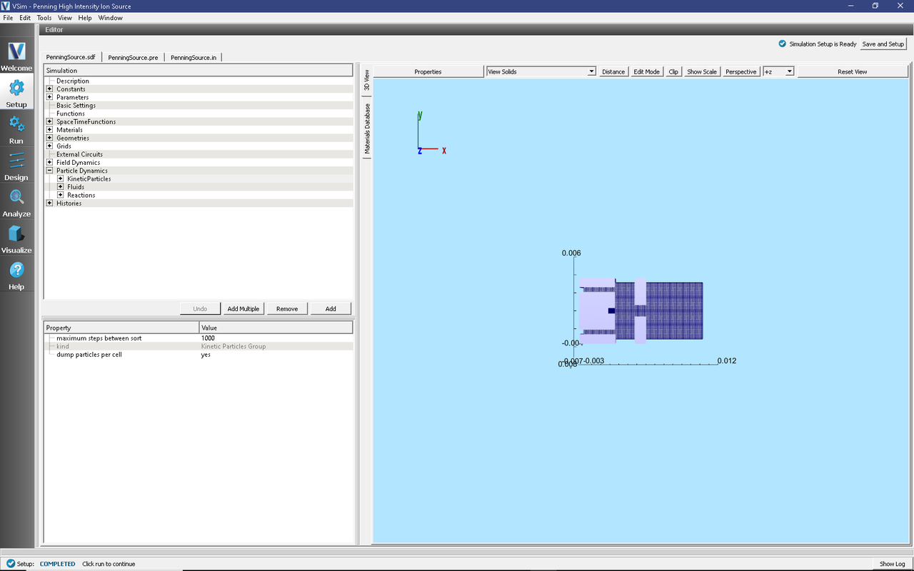
Fig. 558 Location of the flag to turn on tracking and dumping the number of particles per cell.

Using the Analyzer to Create a Custom Decomposition

After turning on tracking the PPC for the simulation, and running it. There should be a dump file with the naming scheme: simulationName_speciesPPC_dumpNumber.h5 Once there is, continue as follows:

• Proceed to the Analysis Window by pressing the Analyze button in the navigation column.

• In the resulting list of Available Analyzers, select computeLoadBalancedDecomp.py and press Open

• The analyzer fields should be filled as below:

  • simulationName: PenningSource

  • species: Blank. Typically will be “electrons” or “Ar” which are the names of the two species in the “Particle Dynamics” tab in the visual setup.

  • nnodes: Blank. This value is 1, unless using more than one node on a HPC.

  • ncores: Blank. This value is the number of cores you would like to use.

  • periodic_dirs: 2. This example has 2 periodic boundaries.

  • dump_number: 0. This is the dump you wish to perform the analysis upon. Preferably the most recent one.

• Note, unless you wish to have slab decomposition, leave intra- & inter-slice unchecked.

• Click Analyze in the top right corner.

• The analysis is completed when you see output similar to that shown in Fig. 559.

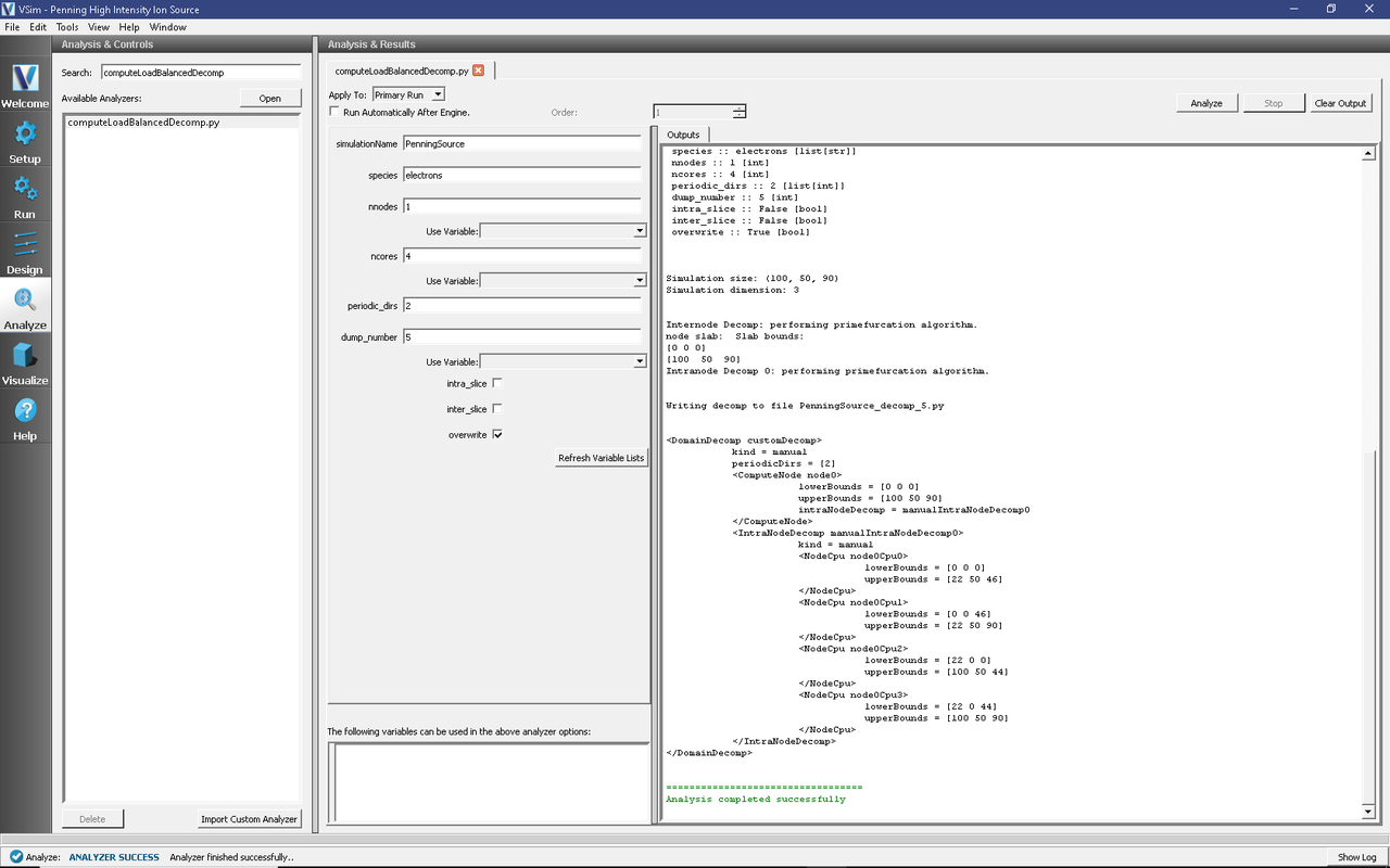
Fig. 559 Output of the computeLoadBalancedDecomp analyzer for a 32 core run on 1 node (i.e. workstation or 1 node of a hpc) at time step 5000.

Along with the screen readout, the analyzer also writes a file to disk, with the naming convention <simulationName>_decomp_<dumpNumber>.mac, using values from their respective fields.

Loading the Custom Decomposition into the Simulation

This custom decomposition file can be loaded into VSimComposer to then be used. To do this, proceed as follows:

• Proceed to the Setup Window by pressing the Setup button in the navigation column.

• In the Simulation sub-pane of the sdf, Expand the Basic Settings option.

• Select the domain decomposition property to see the drop-down menu.

• Select manual

• Enter the filename of the custom decomposition file. If from the analyzer, recall it has a form of <simulationName>_decomp_<dumpNumber>.mac

This is shown in Fig. 560.

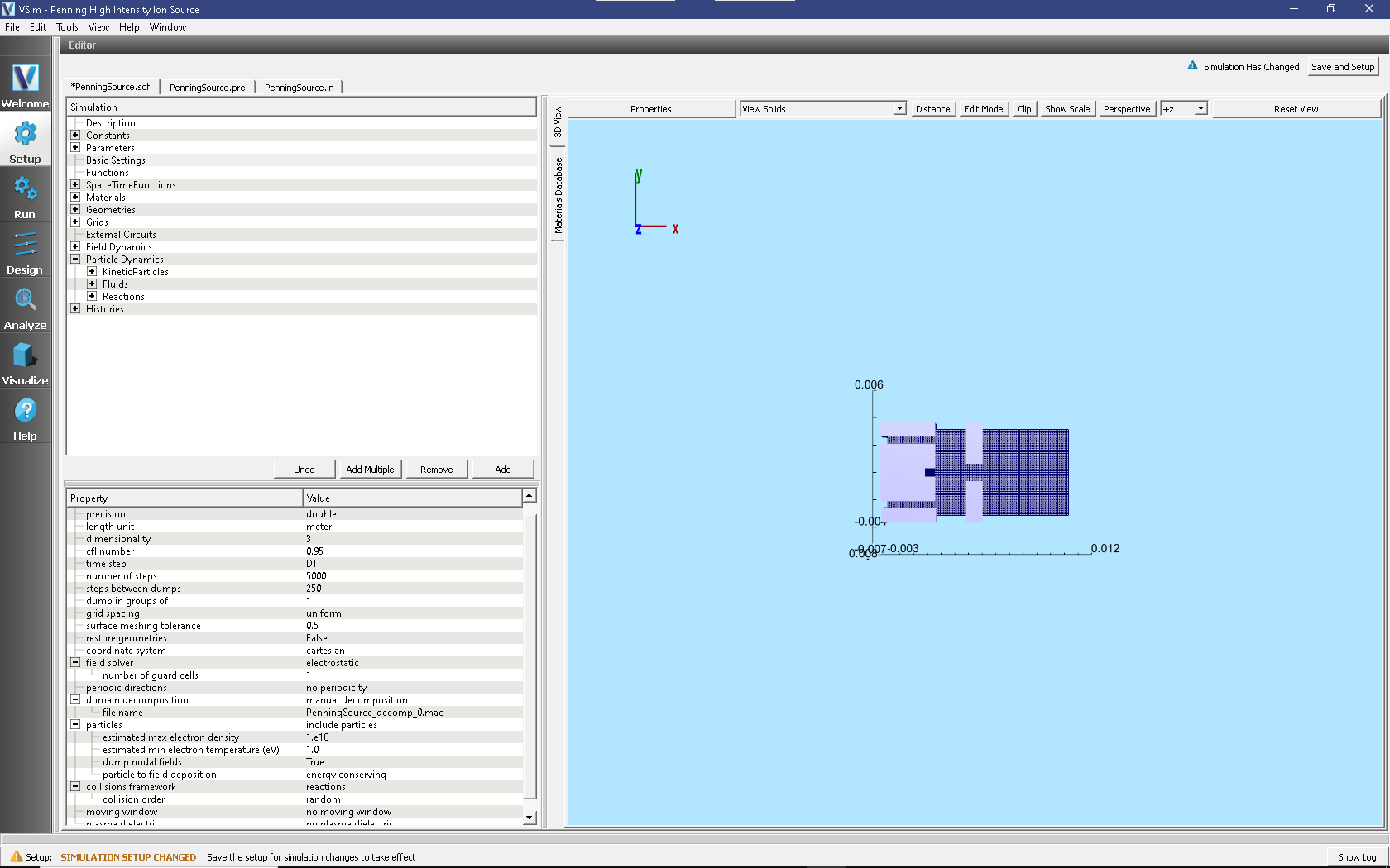
Fig. 560 Location of the drop-down menu to import a custom decomposition file.

References

[1] Birdsall, C. K., & Langdon, A. B. (1985). Plasma Physics via Computer Simulation. New York: McGraw-Hill.