Negative Ion Beam (negativeIonBeam.sdf)
Keywords:
- ion beam, beam transport, reactions, electrostatic
Problem description
VSim may be used to model ion beam transport and particle dynamics where the beam is represented by kinetic simulation particles. Low density background gasses can cause instabilities in the beams due to collisions between the beam particles and the background gas.
In this simulation, a beam of H- ions propagates through a background H2 gas. Collisions between the beam ions and the background gas produce electrons, H2+, and neutral H through the following reactions:
\(H^- + H_{2} \rightarrow H^{-} + H_{2} ^+ + e^-\) (ion impact ionization)
\(e^- + H_{2} \rightarrow H_{2} ^+ + 2e^-\) (electron impact ionization)
\(H^- + H_{2} \rightarrow H + H_{2} + e^-\) (detachment)
\(H^- + e^- \rightarrow H + 2e^-\) (stripping)
There are other reactions that are not included in this tutorial simulation. Typically these reactions have low cross sections. Fig. 564 shows the cross sections for the above reactions as a function of incident energy.
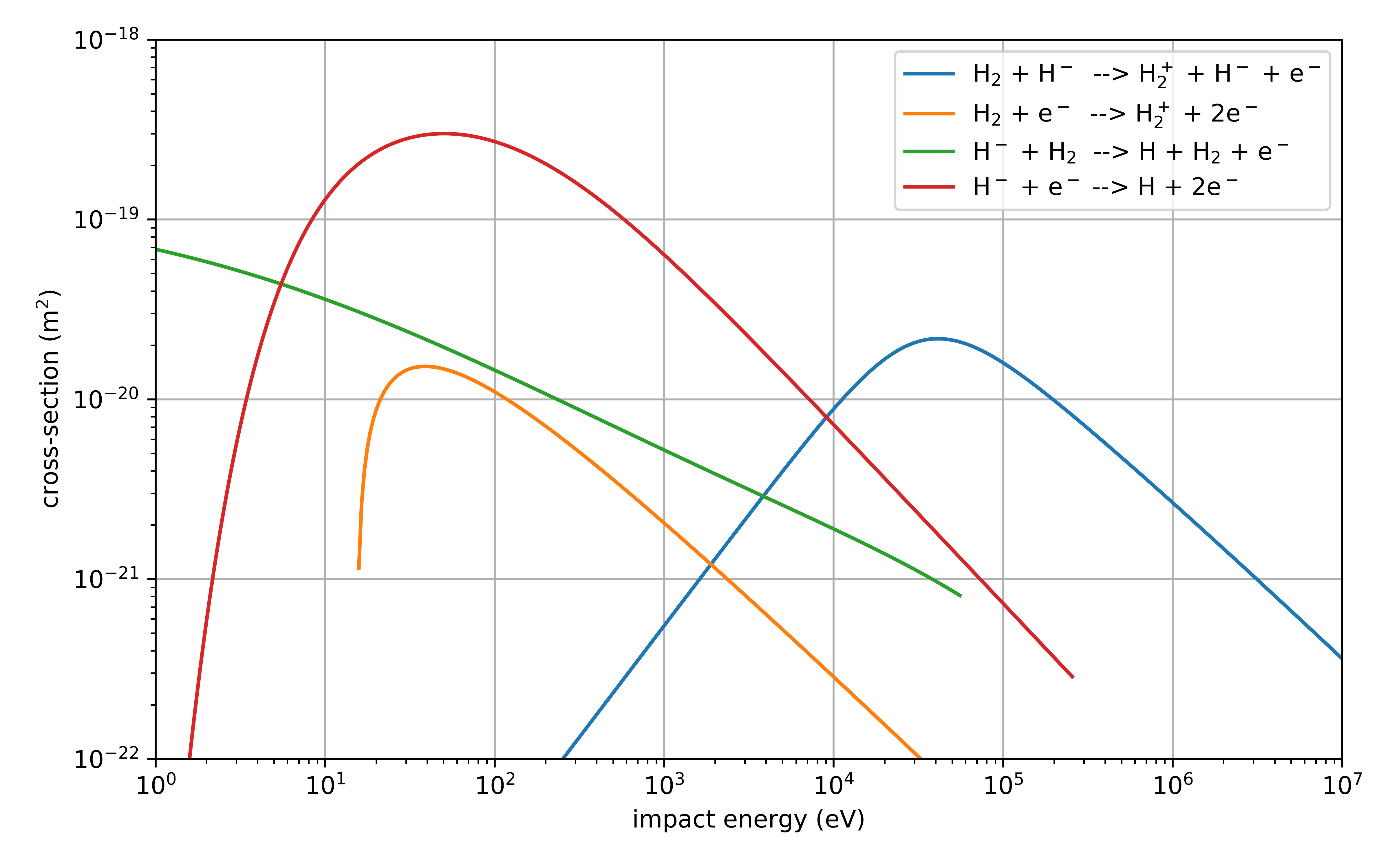
Fig. 564 Cross sections for the four collision reactions included in this example.
This simulation can be performed with a VSimPD license.
Opening the Simulation
The Kinetic Collisions example is accessed from within VSimComposer by the following actions:
Select the New → From Example… menu item in the File menu.
In the resulting Examples window expand the VSim for Plasma Discharges option.
Expand the Processes option.
Select “Negative Ion Beam” and press the Choose button.
In the resulting dialog, create a New Folder if desired, and press the Save button to create a copy of this example.
The Setup Window is now shown with all the implemented physics and geometries, if applicable. See Fig. 565.
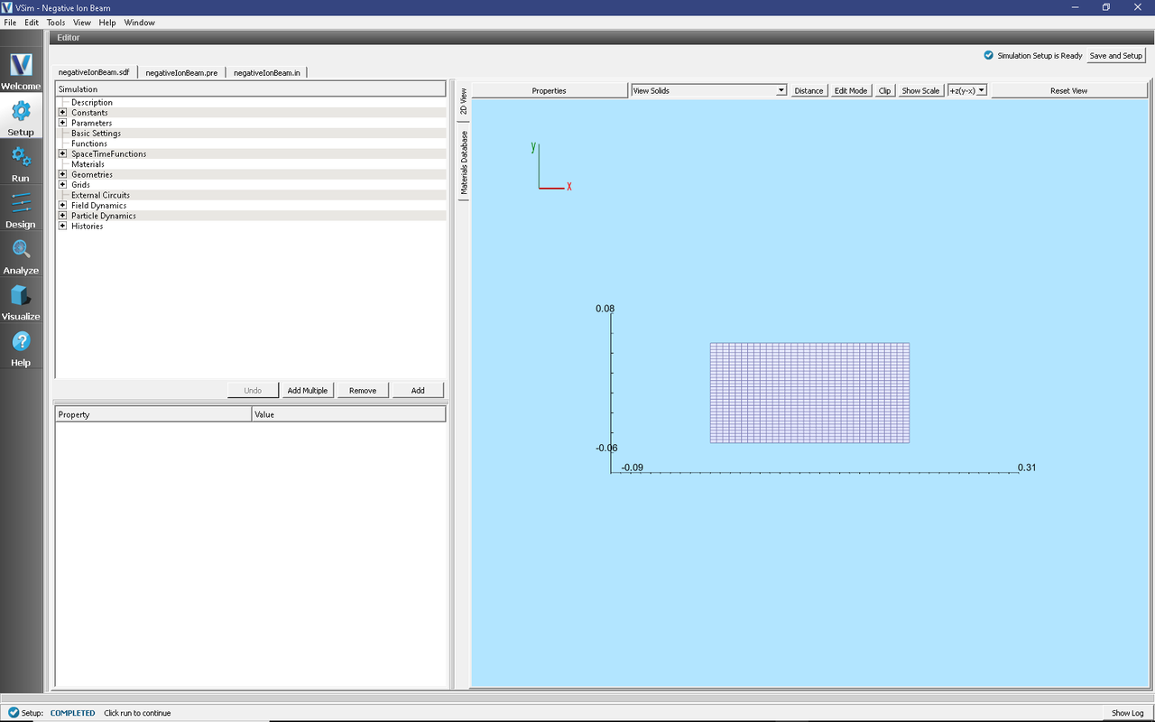
Fig. 565 Setup Window for the Negative Ion Beam example.
Simulation Properties
This input file contains a number of different kinetic species as well as a background fluid description of a gas. Ionization collisions between kinetic particles and the background gas are described by Monte Carlo interaction blocks of kind impactIonization, and detachment of electrons due to a collision with the background gas are of kind negativeIonDetachment. Collisions between kinetic particles and other kinetic particles are described in the input file by an interaction of kind binaryIonization.
The fields are electrostatically solved for at each time step, including the fields due to all charged particles, subject to the boundary conditions specified in the input file. There are a number of histories that record the number of particles for different species, their energies, as well as currents absorbed at the boundaries.
Running the Simulation
After performing the above actions, continue as follows:
Proceed to the Run Window by pressing the Run button in the left column of buttons.
To run the file, click on the Run button in the upper left corner of the Logs and Output Files pane. You will see the output of the run in this pane. The run has completed when you see the output, “Engine completed successfully.” This is shown in the window below.

Fig. 566 The Run Window at the end of execution.
Analyzing the Results
If it is desired to calculate the density of the electrons the analysis script computePtclNumDensity.py must be used.
First click on the Analyze Tab.
From the list of Available Analyzers and choose computePtclNumDensity.py. Then click Open at the bottom of the Analysis Controls pane.
Ensure that the “simulationName” field is “negativeIonBeam” and enter “Electrons” in the “speciesName” field. Leave the “aveNxN” and “iterateAve” with their default values.
Press the Analyze button on in the upper right corner of the window to run the analysis. Below, the Analyze Tab is shown at the end of a successful run.
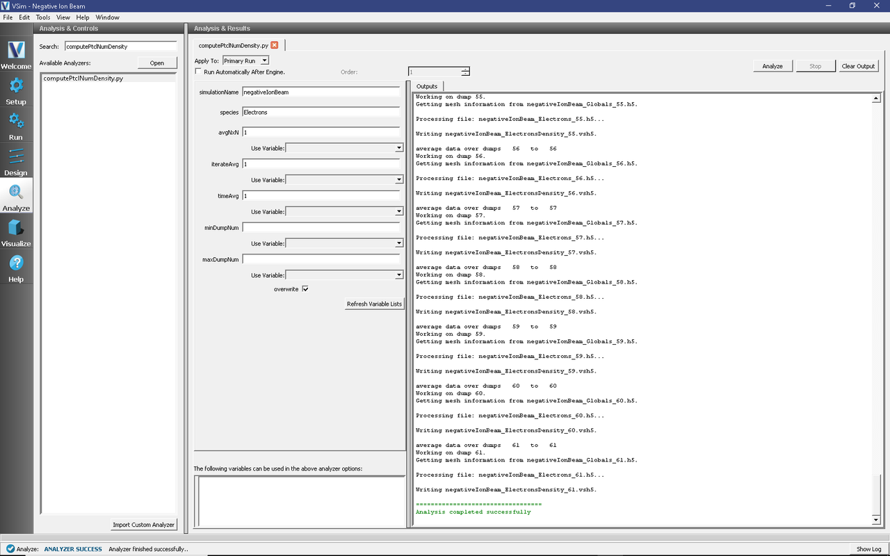
Fig. 567 The Analyze Window at the end of execution.
The resulting data can be visualized as “ElectronsDensity” under the Scalar Data menu in the Visualize Tab. A plot of this data is shown below in Fig. 568. The density of H2plus, Hminus or Hneutral can also be calculated if those species names are used in place of “Electrons” and the analyzer is re-run. If you have previously navigated to the Visualize Tab, you will need to press the Reload Data button at the bottom of the Visualize Tab to view the data.
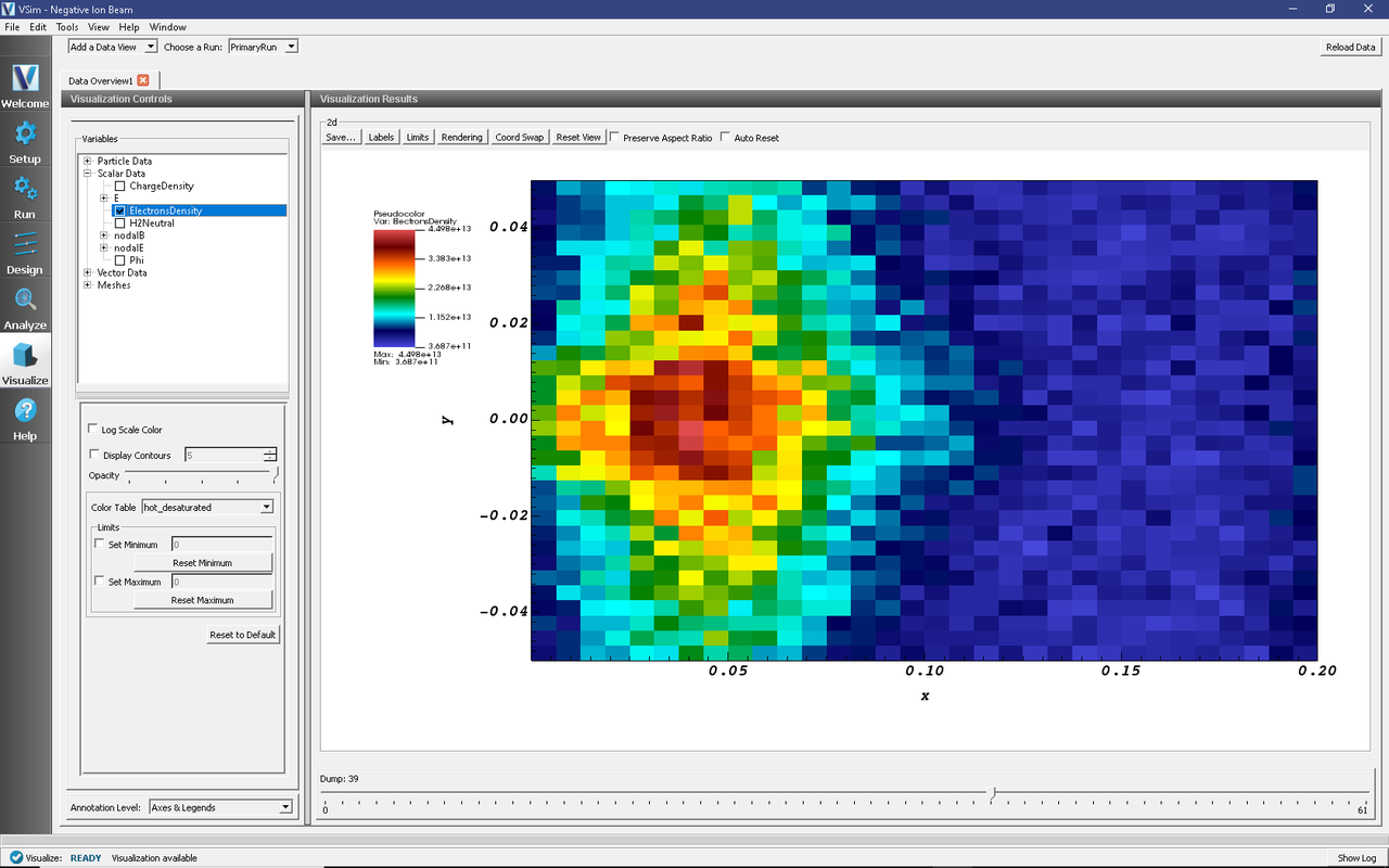
Fig. 568 Plot of the electron density at dump 39.
Visualizing the Results
After performing the above actions, continue as follows:
Proceed to the Visualize Window by pressing the Visualize button in the left column of buttons.
Expand “Particle Data” and select “Electrons,” “H,” “H2Plus,” and “Hminus”.
Then expand “Scalar Data” and select “Phi.”
Check the Display Contours” box, which is below the *Variables box in the Visualization Controls pane.
Set the “# of Contours” to 20. The scroll through the dumps to produce the image in Fig. 569.
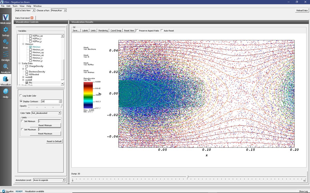
Fig. 569 Visualization of particle densities as a color contour plot, overlaid with a scatter plot of the particle positions.
Further Experiments
The background gas pressure is higher than one would typically see in an accelerator in this example so that the example will produce results quickly. Decreasing the pressure will give the same results, but over longer time scales.
Since this beam is negatively charged, it repulses electrons from the region near the beam. Decreasing the beam current will produce more neutralizing H2+ near the beam as the electrons can more effectively ionize the background H2 gas in that area.