Cylindrical Hall Thruster (cylHallThruster.sdf)
Keywords:
- electric propulsion, Hall thruster channel, erosion models.
Problem description
Electric Hall thrusters are used for in-space propulsion and satellite station-keeping needs. The discharge plasma inside the Hall thruster channel is produced by the ionization of electrons with a neutral propellant gas such as xenon. The electrons are emitted from the neutralizer cathode placed at the exit of the Hall thruster (cathode end). The neutral gas is fed into the channel from the anode end of the Hall thruster channel. The electrons are confined inside the Hall thruster channel by the radial magnetic field applied through the solenoidal magnetic fields. Plasma xenon ions are accelerated out of the channel at high velocity, which produces the thrust necessary for space propulsion. Recently these thrusters are being designed to support long life time, high-power and high-thrust operations. The channel wall erosion occurring inside of the Hall thruster is one of the main limitations to these design needs. It becomes important to understand the plasma discharge processes occurring inside the Hall thruster channel and predict the lifetime of the Hall thruster based on the calculations of sputtered material from the Hall thruster channel.
This example demonstrates the xenon discharge plasma processes of a Stationary Plasma Thruster (SPT-100) channel. The outer cylinder has a radius of 5 cm and the inner cylinder has a radius of 3.5 cm. The radial channel gap is 1.5 cm. The channel length is 2.5 cm and our simulation domain is extended up to 1 cm outside the channel region (to simulate both channel and plume plasma). The left wall is biased at 300 V anode potential. Both inner and outer cylinders are maintained as dielectric cylinders (with hexagonal boron-nitride dielectric material coating) with a dielectric permittivity ratio of 4.6. The exit boundary is taken at 0 V. An electron source is placed at the channel exit for considering the electron emission from the neutralizer cathode. The cathode emission current is taken as 4.5 A. The xenon neutral gas is considered as a static fluid background. The neutral gas density is taken to be linearly decreasing trend with a maximum gas density is taken at the anode end of the channel. The simulation is initiated from a uniform plasma with both electrons and xenon ions. We enable a self-similar scaling system laws for the simulation of Hall thruster channel described by figure 1 in [Mahalingam2011]. This is based on earlier work by Taccogna [Taccogna2005] [Taccogna2004]. We have taken a scale factor of 1/50, i.e., the thruster dimensions are scaled by 1/50. This scaling is followed so that the kinetic Hall thruster channel plasma simulations can be performed in a reasonable run time. The scaling affects the physical dimensions and external potentials.
This example does demonstrate ionization of neutral fluids in cylindrical geometry.
This simulation can be performed with a VSimPD license.
Opening the Simulation
The Cylindrical Hall Thruster example is accessed from within VSimComposer by the following actions:
Select the New → From Example… menu item in the File menu.
In the resulting Examples window expand the VSim for Plasma Discharges option.
Expand the Spacecraft option.
Select Cylindrical Hall Thruster and press the Choose button.
In the resulting dialog, create a New Folder if desired, and press the Save button to create a copy of this example.
All of the properties and values that create the simulation are now available in the Setup Window as shown in Fig. 596.
You can expand the tree elements and navigate through the various properties, making any changes you desire.
The right pane shows a 3D view of the geometry, if any, as well as the grid, if actively shown.
To show or hide the grid, expand the Grid element and select or deselect the box next to Grid.
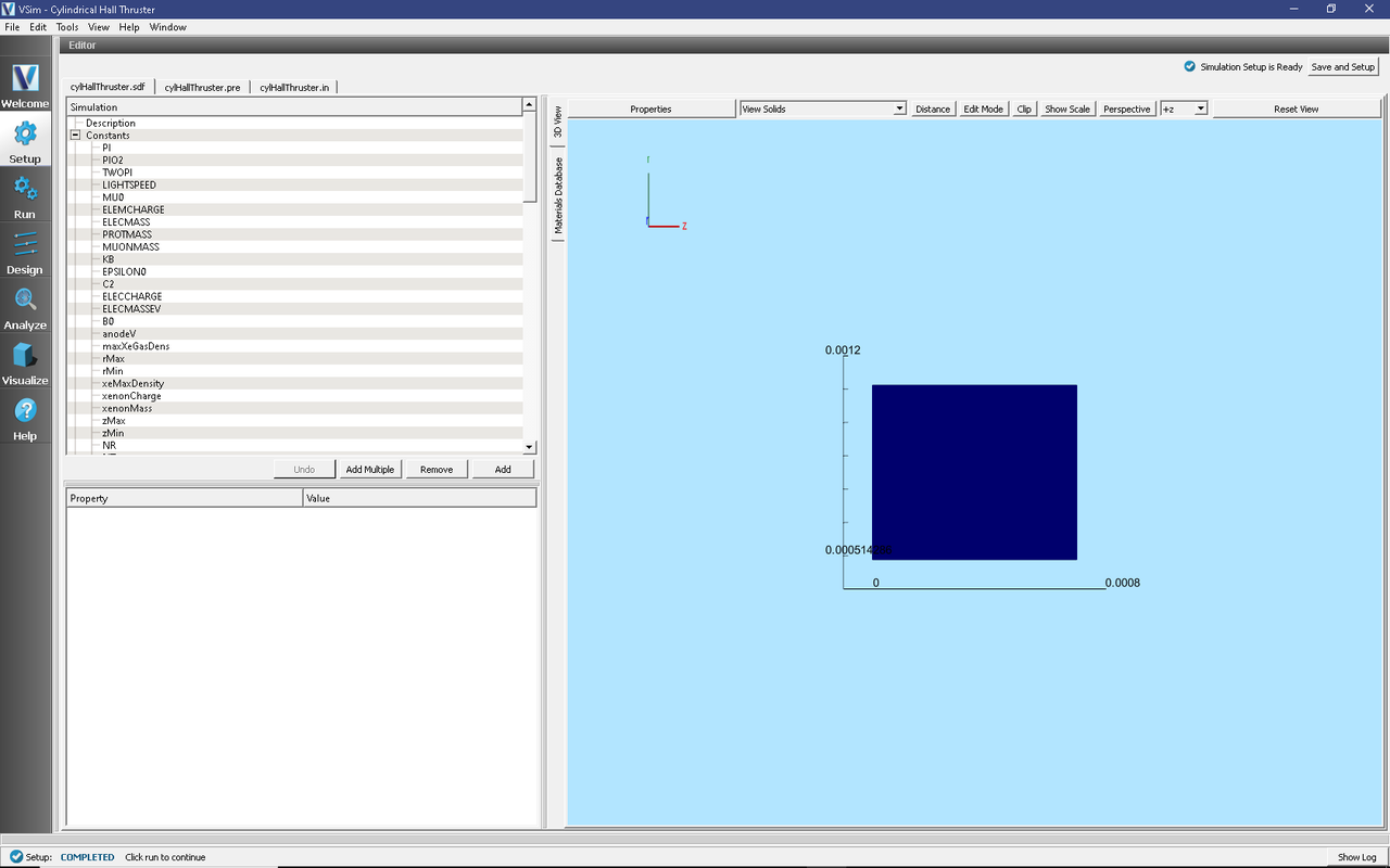
Fig. 596 Setup Window for the Cylindrical Hall Thruster Channel example.
Simulation Properties
This example contains many user defined Constants which help simplify the setup and make it easy to modify. These include constants such as:
B0: The amplitude of the background magnetic field
anodeV: the anode voltage
innerRad and outerRad: inner and outer cylinder radius
xeMaxDensity: the maximum density of the background Xe fluid
There are also several SpaceTimeFunctions that are used to define spatially and/or temporally varying inputs to other properties. These include:
By: the magnetic field profile
initialGasDensity: the profile for the background gas density
The self-consistent electric field is solved from Poisson’s equation by the electrostatic solver in a cylindrical coordinate system. The simulation is performed in axisymmetric 2-D fashion. The plasma is represented by macro-particles which are moved using the Boris pusher in cylindrical coordinate system. Various types of elastic and inelastic collisions of the particles are also taken into account.
Running the simulation
After performing the above actions, continue as follows:
Proceed to the Run Window by pressing the Run button in the left column of buttons.
To run the file, click on the Run button in the upper left corner of the Logs and Output Files pane. You will see the output of the run in this pane. The run has completed when you see the output, “Engine completed successfully.” A snapshot of the simulation run completion is shown in Fig. 597.
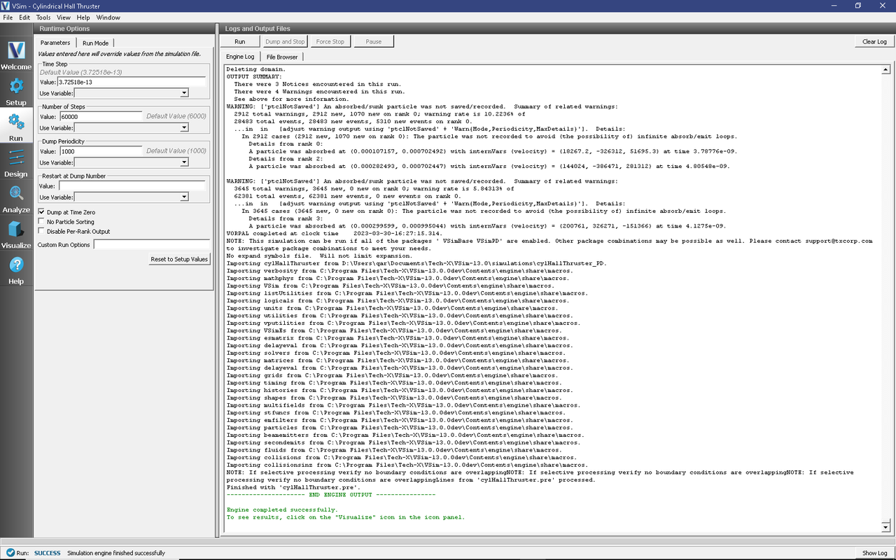
Fig. 597 The Run Window at the end of execution.
Analyzing the Results
If it is desired to calculate the density of the electrons or ions the analysis script computePtclNumDensity.py must be used.
First click on the Analyze Tab.
From the Available Anaylzers list, choose computePtclNumDensity.py. Then click Open.
This script accepts the simulationName (Name of the input file) and speciesName to be calculated (species of particles).
To calculate the density of the electrons, set the simulationName to “cylHallThruster” and the speciesName to “electrons”.
Click on the Analyze button at the top right of the Analysis Results pane.
A snapshot of the simulation run completion is shown in Fig. 598.
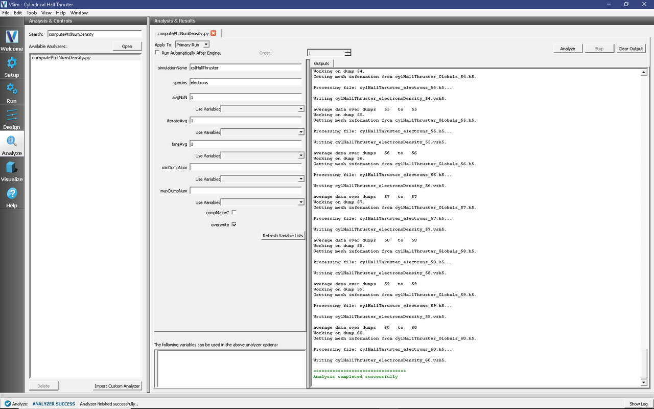
Fig. 598 The Analyze Window at the end of execution.
The resulting data will be visualizable as electronsDensity under the Scalar Data menu in the Visualize Tab. The density of other particles such as heavyIons, or Xeplus can also be calculated if those species names are used in place of electrons.
Visualizing the Results
To visualize the results, continue as follows:
Proceed to the Visualize Window by pressing the Visualize button in the left column of buttons.
There are many different fields, particles, and histories that can be visualized in this example. The horizontal axis represents Z direction and the vertical axis represents R direction.
To view the electric potential, click on “Add a Data View” in the upper left corner of Composer. Then click on “Field Analysis”. This will open a new field analysis tab. In the new tab, click on the down arrow next to “Field” and choose “Phi”. Scroll the dump slider to view the potential at different times. In the Field Analysis tab, you can view the data as a 2D color contour plot and also look at slices of the data. Fig. 599 shows the visualization seen for the electric potential of the cylindrical Hall thruster channel and in the exit region.

Fig. 599 Visualization of the cylindrical Hall thruster electric potential with a line-out showing the axial sheath structure.
In the Hall thruster channel plasma, the electrons injected from the right end (i.e., exit of the channel) are accelerated towards the anode biased wall at the left end. In VSim it is possible to plot particle data superimposed with a field quantity. To plot both particles and fields, click on “Add a Data View” and select “Data Overview”. In the “Data Overview” tab, expand Scalar Data and select “Phi”. Next expand “Particle Data” and select the “electrons” and “XePlus” check boxes. To view particle data superimposed with field data, it is best to use black and white particles. Therefore, choose the electrons to be white and the XePlus ions to be black. Finally, scroll the dump slider to dump 60 to view the evolved plume and sheath which develops to the right. The figure below, Fig. 600, shows the spatial distribution of positively charged xenon ions (black dots), electrons (white dots) and potential.
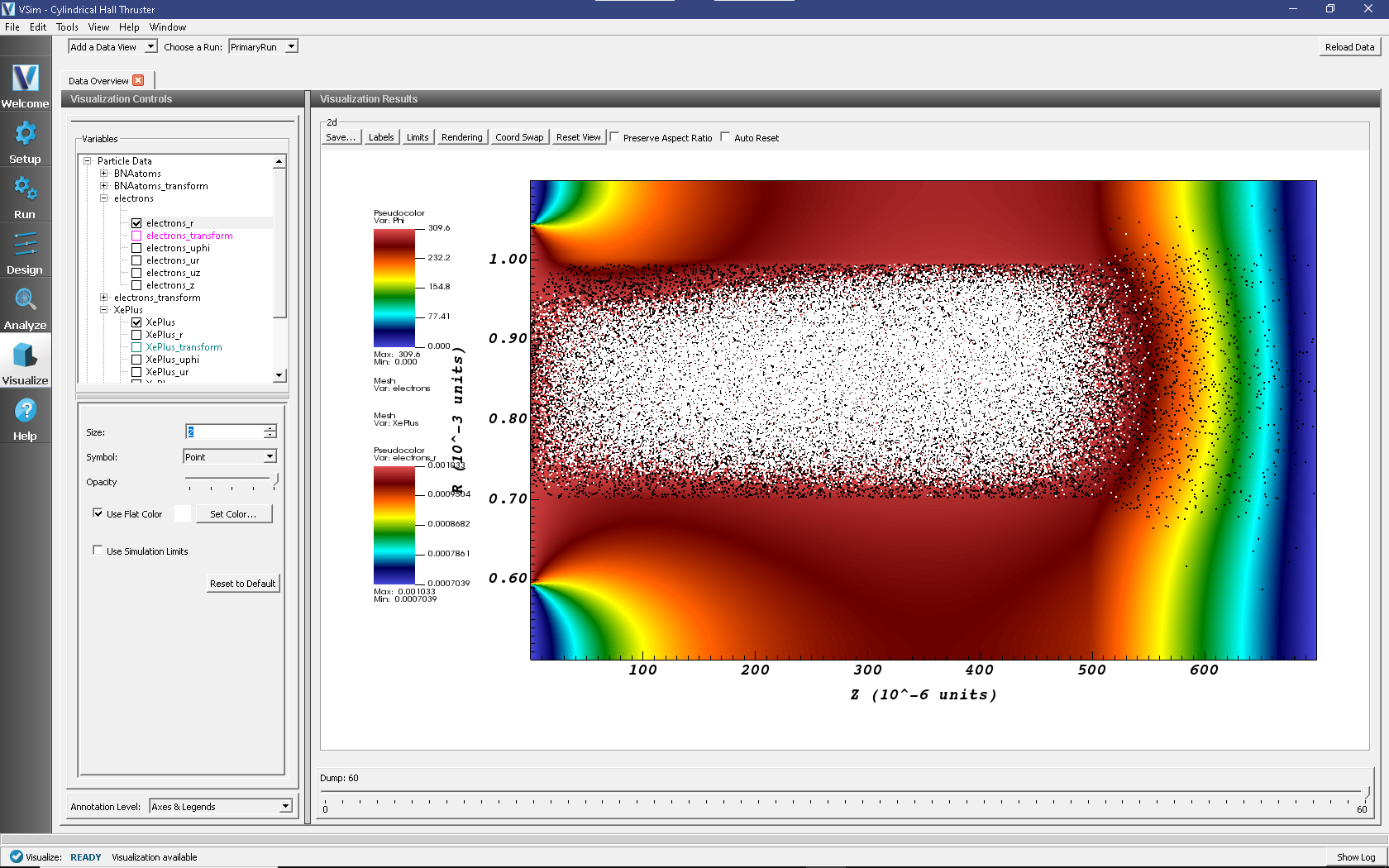
Fig. 600 Visualization of electrostatic potential with the spatial distribution of electrons and ions superimposed.
The static radial magnetic field distribution considered for the SPT-100 Hall thruster channel set up is shown in Fig. 601. To reproduce this plot, Open a new Field Analysis tab, click on area next to the Field option, and choose “nodalB_r”. Slide “intercept” to the right so that the lineout goes through the region of the strongest magnetic field. The magnetic field is strong near the inner cylinder and has a Gaussian bell-shaped field distribution both inside and at the exit of the channel.
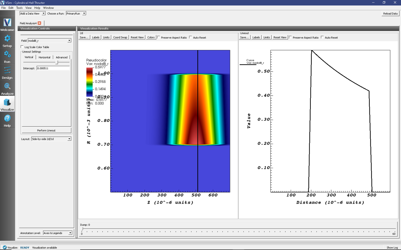
Fig. 601 Visualization of radial magnetic field in the Cylindrical Hall thruster channel. The left panel shows the color contour plot and the right panel shows the lineout.
The background xenon neutral fluid density distribution (plottable as XeNeutralFluid in a Field Analysis tab) used in the simulation set up is shown in Fig. 602. The maximum neutral fluid density is taken at the left end of the channel near the anode wall. A linearly varying neutral fluid density is assumed.
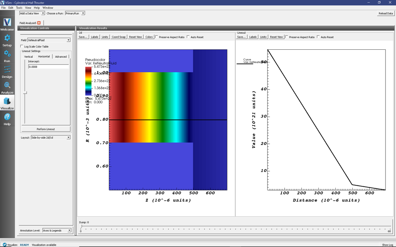
Fig. 602 Visualization of xenon neutral fluid density in the Cylindrical Hall thruster channel.
Finally, we show the electron current impacting the anode and the ion current exiting through the plume. These data are saved in histories called “electronAnodeCurrent” and “absorbedIonCurrent” which are setup in Composer. To view how the histories are created, click on “Setup” on the left hand side of Composer. “Histories” is the bottom-most option in the elements tree. By expanding “Histories” you will see multiple histories already created including “electronAnodeCurrent” and “absorbedIonCurrent”. To view the data, click on “Visualize”. Then click on “Add a Data View” and choose “History”. In the History tab click on “Add Curve” and choose “AbsorbedIonCurrent”. Once the data are plotted, you can add “AbsorbedAnodeCurrent” by clicking on “Add Curve” again and following similar steps.
The resulting data plot is shown in Fig. 603.
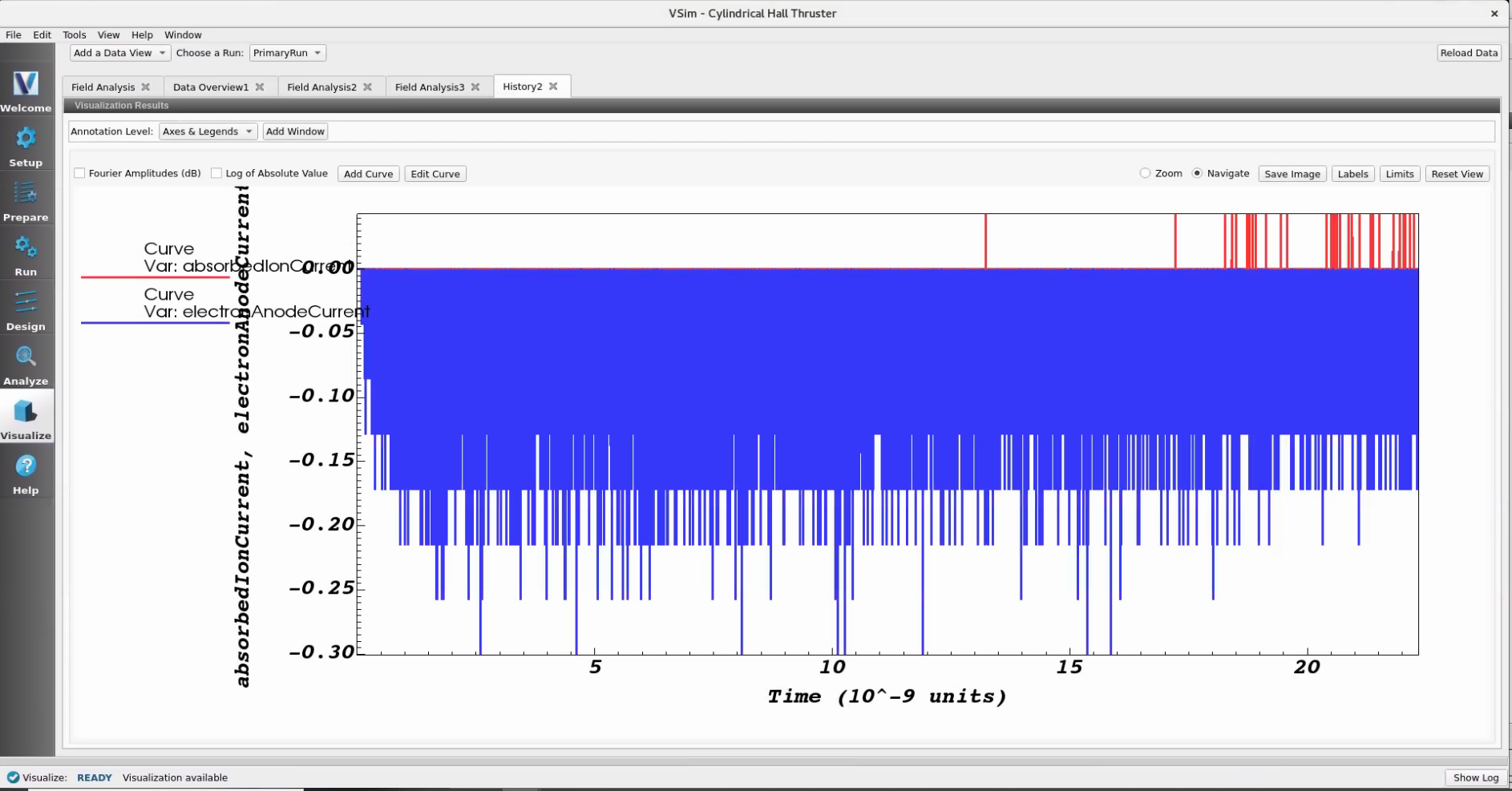
Fig. 603 Visualization showing electron current impacting the anode and ion current leaving through the plume.
Further Experiments
This example can be modified to test different design parameters such as varying anode voltages, varying background neutral gas densities and varying electron emission currents. This will allow users to study high-to-low power and high-to-low throttle levels.
Also the background fluid type can be changed to investigate other fluid species’ in this simulation set up.
{Mahalingam, S., Choi, Y., Loverich, J., Stoltz, P., Bias, B., and Menart, J., “Fully Coupled Electric Field/PIC-MCC Simulation Results of the Plasma in the Discharge Chamber of an Ion Engine,” 47th AIAA/ASME/SAE/ASEE Joint Propulsion Conference & Exhibit, 6071, 2011.
Taccogna, F., Longo, S., Capitelli, M., and Schneider, R., “Plasma Flow in a Hall Thruster,” Physics of Plasmas, 112, 2005.
Taccogna, F., Longo, S., Capitelli, M., and Schneider, R., “Stationary plasma thruster simulation,” Comp. Phys. Comm., 165, pp. 160-170, 2004.