Ion Thruster (ionThrusterT.pre)

Keywords:

electric ion thruster discharge chamber plasma processes in 2D cylindrical system.

Problem Description

Ion thrusters are electric propulsion devices used for in-space propulsion and satellite station-keeping. In this device, a propellant gas (xenon in this example) is ionized into a plasma state inside a cylindrical discharge chamber. The plasma ions are accelerated out of the chamber through an electrostatic grid optics system to produce thrust. The device consists of the following components: an anode-biased discharge chamber, a discharge hollow cathode assembly, permanent magnet rings, a neutral propellant feed system, grid optics (screen and accelerator plates), and a neutralizing hollow cathode. The discharge hollow cathode is placed in the center of the discharge chamber and emits energetic electrons (primary electrons) into the system. Primary electrons undergo ionizing collisions with the neutral propellant gas inside the chamber to produce plasma ions and secondary electrons. An energetic electron impacting a xenon atom that is already singly ionized may cause another electron to detach, resulting in a doubly ionized xenon atom. The permanent magnetic rings within the discharge chamber confine the electrons, increasing their time of flight in the chamber, and thus their chances of ionizing neutrals before collection at the anode-biased discharge chamber walls. The plasma ions produced in the chamber leave primarily through the screen grid plate with some losses to the cathode biased walls. To ensure long discharge cathode lifetimes, a protective enclosure called a cathode keeper (generally kept between 3 and 5 volts above the discharge cathode voltage) is used to shield the cathode plate from plasma ion collisions. The bombardment of singly charged and doubly charged ions during thruster operation will over time erode the face of the cathode keeper and expose the discharge cathode to energetic ions. Thus, it becomes important to model the ion flux around the cathodes. Recently ion thrusters have been designed to meet high-power and high-thrust-to-power space propulsion requirements. Numerical discharge chamber plasma simulations provide a detailed understanding of the plasma processes that go on inside a discharge chamber and help with the calculation of electron discharge currents, ion beam currents, and ion current losses to the chamber walls.

This example demonstrates the xenon discharge plasma processes inside of a cylindrical discharge chamber with a three-ring magnetic circuit arrangement. One magnetic ring is mounted on the forward wall (seen as the left wall in the geometry of the example) and two magnetic rings are mounted to the exterior wall of the cylindrical discharge chamber (seen as the top wall in the example setup). The radius of the cylindrical chamber is 20 cm and it is 18 cm long. The screen grid plate has a radius of 18 cm and is placed at the aft end of the discharge chamber (far right in the example setup). The discharge hollow cathode assembly is placed at the center of the discharge chamber. The radius of the cathode keeper assembly is taken to be 0.75 cm and its orifice protrudes out 7 cm from the forward wall (from the left wall in the example diagram). An electron particle source is implanted next to the cathode keeper orifice to model the electron emission of the discharge cathode. In this simulation the cathode emission current is taken as 10 A. The same cathode emission source location is also used for modeling the neutral propellant flow from the discharge cathode. The main xenon neutral propellant source is modelled along the exterior wall (top wall in the example diagram). We have taken neutral propellant flow rates of 4.5 sccm and 43.5 sccm for the discharge cathode neutral source and main neutral source respectively. The anode biased discharge chamber walls are kept at 25 V. The discharge cathode keeper is biased at 5 V and the screen grid plate is kept at 0 V. Finally, we enable a self-similar scaling system for the simulation of discharge chamber plasma described by figure 1 in [MCL+11]. This is based on earlier work by Taccogna [TLCS04, TLCS05]. By default the shrink scale factor is 200, i.e., the thruster dimensions are scaled by 1/200. This scaling ensures that simulations can be performed in a reasonable run time but it requires use of an inflated permittivity scale factor, i.e. the permittivity of free space is artificially inflated so that numerical parameters like grid spacing and time step values satisfy the smaller plasma frequency and Debye length.

The simulation is initiated with the chamber pre-filled with xenon neutrals. This is because the neutrals are heavy and slow, and it would take a great many time steps at the start of every run to populate an empty chamber. To view the initial distribution of neutrals, the input file can be run with particle sources turned-off. To do this, switch the TURN_THRUSTER_OFF parameter to 1 and run for one time step. Then, in the Visualize window, select XeNeutrals under Particle Data.

This simulation can be performed with a VSimPD license.

Opening the Simulation

The ion thruster example is accessed from within VSimComposer by the following actions:

• Select the New → From Example… menu item from the File menu.

• In the resulting Examples window expand the VSim for Plasma Discharges option.

• Expand the Spacecraft (text-based setup) option.

• Select Ion Thruster (text-based setup) and click the Choose button.

• In the resulting dialog, create a New Folder if desired, and press the Save button to create a copy of this example.

The basic variables of this problem should now be alterable via the text boxes in the left pane of the Setup Window, as shown in Fig. 612.

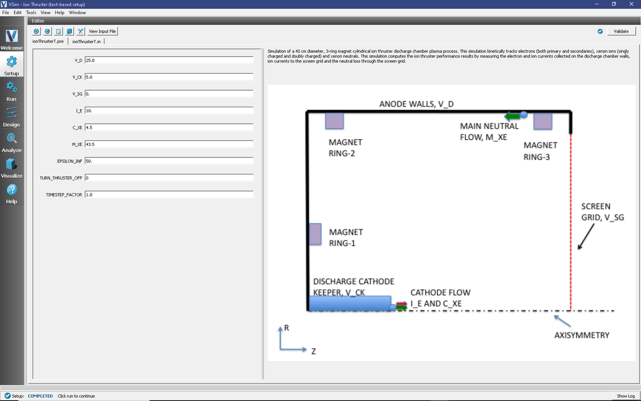
Fig. 612 Setup Window for the Ion Thruster example.

Input File Features

The input file allows the user a choice of ion thruster operating parameters such as discharge voltage, cathode keeper voltage, screen grid voltage, discharge cathode electron emission current, cathode neutral flow rate, and main neutral flow rate. Also it gives the user an option to specify the inflated permittivity scale factor by which the real permittivity of free space is scaled.

The self-consistent electric field is solved from Poisson’s equation by the electrostatic solver in cylindrical coordinates. Because this simulation is defined in the r-z plane, the Laplacian uses a cylindrical geometry involving a 1/r term in the derivative with respect to r. The simulation is performed in an axisymmetric 2-D (r-z) domain. The actual thruster dimensions are reduced by the SHRINK_FACTOR variable in the input file (default 200). Correspondingly the physical parameters such as electric fields, magnetic fields, and particle densities are scaled by the shrink factor to maintain consistent physical effects (e.g. Larmor radius, Knudsen number).

The plasma is represented by macro-particles which are moved via the Boris pusher in cylindrical coordinates. Various types of elastic and inelastic particle collisions are calculated with the computational engine’s Monte Carlo package. In this simulation the propellant xenon neutrals are tracked as kinetic particles and undergo collisions with electrons. The simulation employs variable-weight particle splitting and self-combination via NullInteraction blocks to help maintain good particle resolution over orders-of-magnitude variations in density across the domain.

This input file contains an imported magnetic field. The external magnetic field file is in units of Gauss, and is converted into Teslas when imported by VSim.

Running the Simulation

After performing the above actions, continue as follows:

• Proceed to the Run Window by pressing the Run button in the left column of buttons.

• Check the box labeled “Dump at Time Zero” so that the initial electric potential may be plotted.

• To run the file, click on the Run button in the upper right corner of the window. You will see the output of the run in the right pane. The run has completed when you see the output, “Engine completed successfully.” A snapshot of the simulation run completion is shown in Fig. 613.

The default number of time-steps for this simulation is 5,000, but to approach steady-state, approximately 500,000 time-steps are required. The Visualizing the Results section provides a review of the results at 5,000 time-steps, while the Further Experiments section is a review of the results after 500,000 time-steps.

Fig. 613 The Run Window at the end of execution.

Analyzing the Results

If the electron density is desired the analysis script computePtclNumDensity.py may be used.

• In the leftmost panel, click the Analyze button. Select computePtclNumDensity.py from the list of analyzers, then click Open at the top of the Analysis Controls pane.

• Enter “electrons” into the speciesName field.

• Click the Analyze button near the upper right of the Analysis Results pane.

• Repeat with other particle species if desired (“XeIons”, “XeNeutrals”)

The analysis results are now viewable in the Visualize window, as shown in the following section.

Visualizing the Results

After performing the above actions, continue as follows:

• Proceed to the Visualize window by clicking the Visualize button in the leftmost panel.

• In the top of the Visualization Controls pane, click on the Add a Data View button then click on Field Analysis. This will open a new Field Analysis tab next to the existing Data Overview tab.

• In the Field dropdown menu, select phi. A pseudocolor plot of the potential with a radial lineout performed should be displayed as shown in Fig. 614.

• To plot the axial potential profile, in the Lineout Settings section, select the Horizontal tab, change the intercept to 0.00005, and click Perform Lineout to plot the axial accelerating potential as shown in Fig. 614. If desired, select the Advanced tab to choose arbitrary start and end points for the lineout.

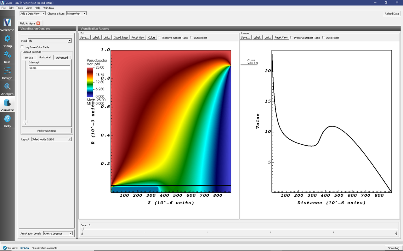
Fig. 614 Visualization of the Field Analysis result for the electric potential inside the ion thruster discharge chamber at timestep 0. Move the slider to the right with your mouse to view advanced timesteps.

• In the top of the Visualization Controls pane, click on the Add a Data View button then click on Phase Space. This will open a new Phase Space tab next to the Field Analysis tab.

• In the Base Variable dropdown menu, select electrons.

• To maintain the same \(z\)-\(r\) convention as the previous electric potential plot, in the X-axis dropdown menu select electrons_z and in the Y-axis dropdown menu select electrons_r.

• Near the bottom of the Visualization Controls pane click DRAW and at the bottom of the Visualization Results pane move the Dump slider to the right to dump 5. The \(z\)-\(r\) phase space should be visible as shown in Fig. 615.

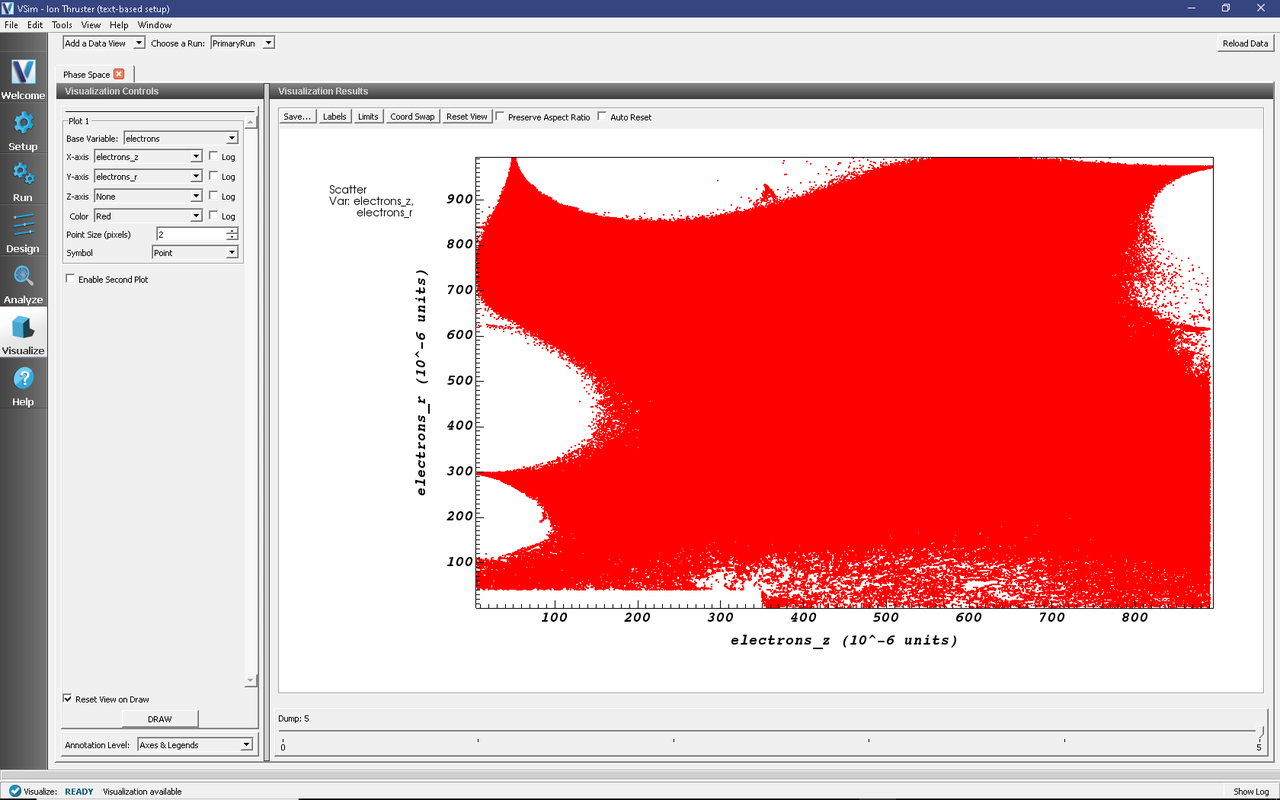
Fig. 615 Electron phase-space distribution results after 5,000 steps.

Recall that the electron number density distribution was calculated in Analyzing the Results. Plot the results of this analyzer as follows:

• In the top of the Visualization Controls pane, switch to the Data Overview tab.

• In the Variables section, expand Scalar Data.

• Select electronDensity. A plot of the electron number density distribution should be displayed, though due to the large variation in densities, only a small portion of the domain will appear to be non-zero

• At the bottom of the variables section of the Visualization Controls pane, select the Log Scale Color checkbox.

• At the top of the Visualization Results pane click the Colors button, and in the resulting dialog set the limits to a minimum of 1e16 and maximum of 1e22, or experiment with limits as desired. The electron density on a logarithmic color scale should now displayed as shown in Fig. 616.

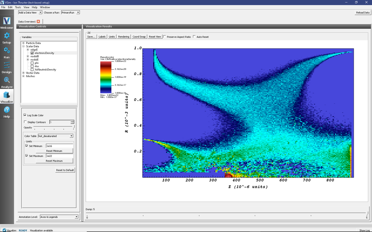
Fig. 616 Electron number density distribution results inside the discharge chamber after 5,000 steps.

Further Experiments

Return to the Run window by clicking on the Run button in the leftmost panel, change Number of Steps to 500,000. To reduce the number of output files, change the Dump Periodicity to 5000 and then click the Run button at the top of the Logs and Output Files pane. A high-performance computing cluster is recommended for this run, which will require approximately 6 days running on 64 cores. When the run has completed, take the following steps.

• Plot the potential at the final data dump similar to the steps taken in Visualizing the Results.

• In the Visualization Results pane, in the 2d section, click the Colors button

• Set the minimum to 0 and the maximum to 25 (Volts). The resulting plot is shown in Fig. 617

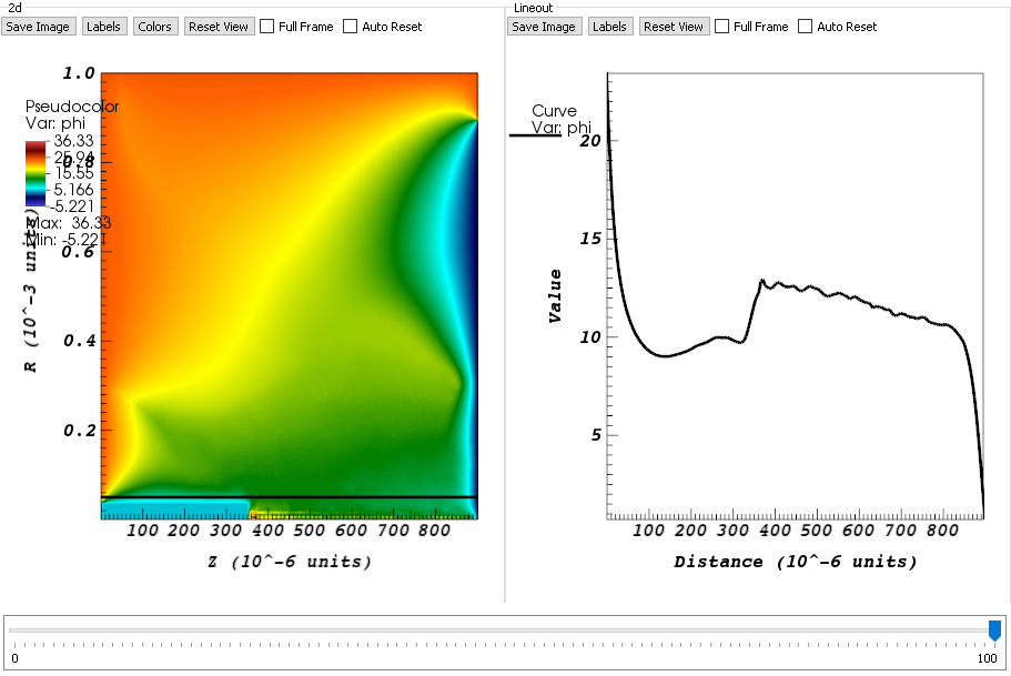
Fig. 617 Electric potential of the plasma inside the ion thruster discharge chamber after 500,000 time-steps.

It can be seen that the ions experience most of their acceleration in the sheath near the right-side boundary of the plasma chamber. Plot the electron and ion densities by taking the following steps:

• Following once again the steps taken in Visualizing the Results, run the computePtclNumDensity.py analyzer on both electrons and XeIons.

• Plot the electrons density using the color log scale and the same limits as previous, as shown in Fig. 618

• Plot the ion density using the color log scale with a minimum of 1e18 and a maximum of 1e23 to get the image shown in Fig. 619 or experiment with the limits as desired.

It can be seen from Fig. 618 and Fig. 619 that the electrons are confined by the magnetic field lines while the much heavier ions are not, allowing a more uniform acceleration of ions out the right side of the chamber, resulting in thrust.

Fig. 618 Electron number density distribution results inside the discharge chamber after 500,000 steps.

Fig. 619 Ion number density distribution results inside the discharge chamber after 500,000 steps.

Plot the electron and ion macroparticle positions with the following steps:

• In the top of the Visualization Controls pane, open a new Phase Space tab under the Add a Data View button.

• Under Plot 1 click the Base Variable drop-down menu and select electrons

• Change X-axis to electrons_z and Y-axis to electrons_r, change Point Size to 1, and at the bottom of the Visualization Controls pane, click DRAW to see the electron macro-particle positions.

• Check the Enable Second Plot button.

• Under Plot 2 change Base Variable to XeIons, change X-axis to XeIons_z and Y-axis to XeIons_r, change Point Size to 1, and click DRAW once again to see the electron and singly-ionized xenon macro-particle positions.

• Check the Enable Third Plot button.

• Under Plot 3 change Base Variable to XeDblIons, change X-axis to XeDblIons_z and Y-axis to XeDblIons_r, change Point Size to 3, and click DRAW once again. The ion and electron positions should be displayed as shown in Fig. 620.

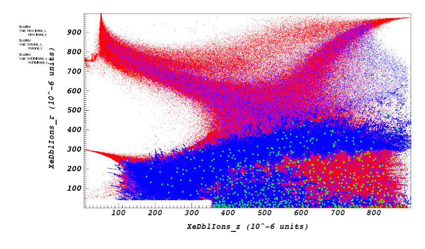
Fig. 620 Electron and ion phase-space distribution results after 500,000 steps.

The electrons appear well confined by the 3-ring magnetic circuit arrangement, and move along the magnetic cusp regions formed between the magnets. Most of the electrons are lost to the discharge chamber walls through the magnetic cusps and are absorbed at the walls in 3 small areas. Only a few electrons are able to cross the strong magnetic field lines and reach the top wall between the cusps.

Singly and doubly ionized xenon are generated inside the discharge chamber through ionizing collisions of electrons with xenon neutrals. Only electrons with energies above the ionization thresholds (12.1 eV for the first ionization level and 21.25 eV for the second) can ionize neutrals.

This input file can be modified to test different design parameters covering a range of anode voltages, xenon flow rates, and electron emission currents, to allow study of high-to-low power and high-to-low throttle levels.