Satellite Surface Charging (satelliteSurfaceChargeT.pre)

Keywords:

electrostatics, surface charges

Problem description

Satellites and other spacecraft operating in the space environment often suffer arcing and breakdown problems due to surface charging. Charged particles buildup on the spacecraft surfaces (such as solar panel arrays and other components) leading to localized arcing/breakdown discharges that can critically fail a component or the entire unit. This problem is made worse as the demand for high power space missions in both satellite and deep-space applications rises. These high-power spacecraft are outfitted with high-voltage solar panels. These panels minimize the overall payload requirements and offer other advantages over more massive, low-voltage arrays. However, they are also more vulnerable to surface charge related arcing. It therefore becomes important to predict the surface charge buildup on spacecraft bodies operating in different space environments, where the ion sources may be natural solar wind or human-made space plasma resulting from electric thruster plasma plumes.

This example demonstrates a satellite body operating in the solar wind environment where the space plasma consists of ions and electrons. The simulation box is set up with dimensions of 15 m x 30 m x 15 m. The satellite system is placed in the middle of the domain. It has a 3 m radius x 5 m long cylindrical central unit connected to solar panels at either end. Each solar panel has a total span length of 7.8 m and a width of 5 m. The satellite central unit has a 5-volt equipotential circular body with radius 2 m and length 3 m. The satellite system is treated as a conductor floating in free space. The system domain boundaries are assumed to have zero perpendicular electric field, i.e. Neumann boundary conditions. The solar wind plasma is introduced in the simulation domain from the positive z direction. The solar wind density is set to \(1 \times 10^{7} \textrm{m}^{-3}\) with a temperature of 10 eV. The number of physical particles per macro-particle is set to 5000. Both electrons and ions are introduced from the source based on the solar wind density and temperature. To maintain plasma uniformity within finite bounds, the electron source rate is inflated slightly because electrons are lighter and leave the system more quickly than do ions. At the same time, the positive ions are imbued with a lighter mass value to speed up the simulation. All simulation boundaries are set up to absorb particles. The charges collected in the satellite system are counted by emitting a heavy electron or heavy ion at the point where an electron or ion was absorbed. The heavy electron/ion is not a physical concept, it is a computational trick whereby any charged particle striking the satellite gets converted to a new species, one with equivalent charge but drastically swollen mass (1 kg in this case) and suppressed energy (suppressed by a factor of 10 billion). In this way, the heavy particles do not propagate from their point of origin, effectively sticking to the satellite surface. To limit the number of macro heavy particles tracked we apply a particle combining algorithm which limits the number of macro particle per cell to one. The collected electron and ion currents on the satellite surfaces are output as histories.

This simulation can be performed with a VSimPD license.

Opening the Simulation

The satellite surface charging example is accessed from within VSimComposer by the following actions:

• Select the New → From Example… menu item in the File menu.

• In the resulting Examples window expand the VSim for Plasma Discharges option.

• Expand the Spacecraft (text-based setup) option.

• Select “Satellite Surface Charging (text-based setup)” and press the Choose button.

• In the resulting dialog, create a New Folder if desired, and press the Save button to create a copy of this example.

The basic variables of this problem should now be alterable via the text boxes in the left pane of the Setup Window, as shown in Fig. 621.

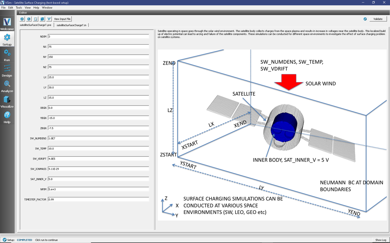
Fig. 621 Setup Window for the Satellite Surface Charging example.

Input File Features

The input file allows a choice of space environment parameters (number density, plasma temperature, drift speed), satellite body voltage, simulation domain size, and resolution (number of cells in each direction).

The self-consistent electric field is solved from Poisson’s equation by the electrostatic solver. The far-field space boundaries are handled with Neumann boundary conditions. The satellite inner body is set up with an equipotential boundary. The surface charges collected on the satellite system make the satellite body float at a slightly higher voltage than the space plasma.

This is a large domain, 3-D problem, and its resolution is aided by several numerical methods. The plasma is represented by macro-particles which are moved according to the Boris pusher. Variable weight particle treatment is employed on all simulated species, reducing the overall number of macro-particles in the computation. Additionally, null interactions are considered as part of the Monte Carlo analysis to limit the number of macro-particles per cell; macro-particles are eliminated in overcrowded cells by means of inelastic combination.

Running the simulation

After performing the above actions, continue as follows:

• Proceed to the run window by pressing the Run button in the left column of buttons.

• To run the file, click on the Run button in the upper left corner of the right panel. You will see the output of the run in the right pane. The run has completed when you see the output, “Engine completed successfully.” This is shown in Fig. 622.

Fig. 622 The Run Window at the end of execution.

Analyzing the Results

If the electron density is desired, then proceed as follows:

• In the leftmost panel, click the Analyze button and then select computePtclNumDensity.py from the list of analyzers, then click Open at the top of the Analysis Controls pane.

• Enter the following parameters in the appropriate fields:

  • simulationName = satelliteSurfaceChargeT

  • speciesName = solarElectrons

  • avgNxN = 1

  • iterateAvg = 1

• Click the Analyze button in the upper right corner of the window.

See Fig. 623.

The resulting data will be visualizable as solarElectronsDensity under the Scalar Data menu in the Visualize Tab. The density of solarIons can be calculated in the same way by substituting that species name in place of solarElectrons.

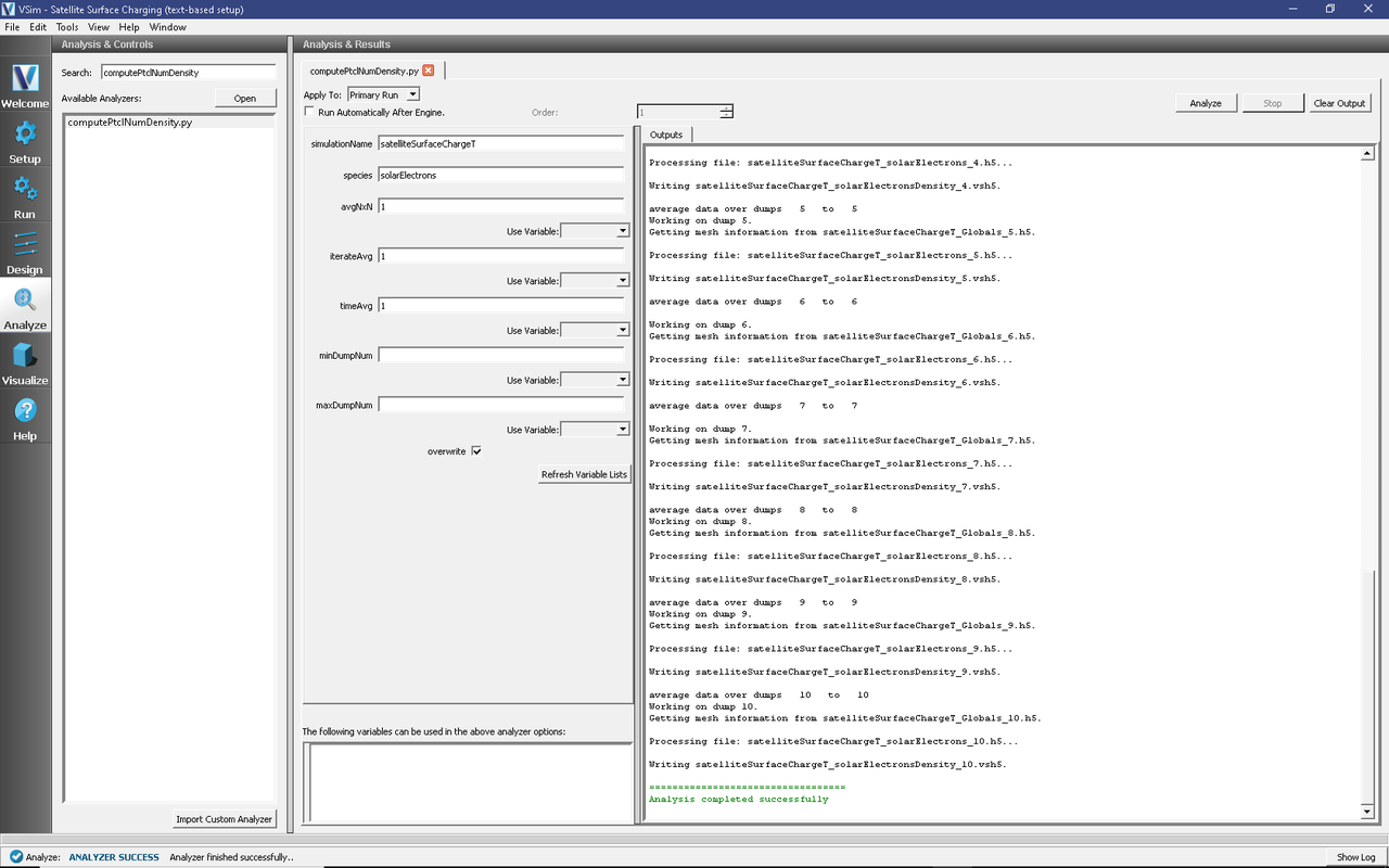
Fig. 623 The Run Window at the end of execution.

Visualizing the results

After performing the above actions, proceed to the Visualize Window by pressing the Visualize button in the left column of buttons.

To visualize the satellite geometry with electrons Fig. 624, proceed as follows:

• Expand Particle Data.

• Expand heavyElectrons.

• Select “heavyElectrons” in red.

• Expand solarElectrons.

• Select “solarElectrons” in green.

• Expand Geometries.

• Select “poly_surface (Satellite)”.

• Move the Dump slider to dump 7.

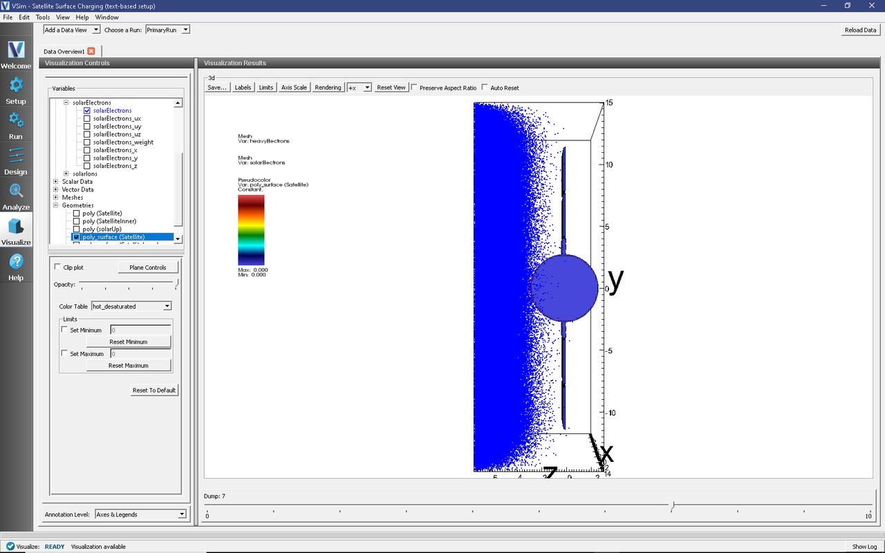
Fig. 624 Visualization plot of satellite system with solar wind electrons in green and the electrons that stick to the satellite surface in red.

Here are some things to try:

• Under Data Overview you can access plots of the electric field, charge density (rho), and electric potential (phi). Select the Display Contours check box for viewing these.

• To view the phase space distribution for the electrons and ions, click on the Data View drop down menu and select Phase Space. Click the Draw button to generate a plot.

• Also from the Data View menu select History to observe the satellite currents and the time history results for the number of macro-particles broken down by species.

To generate Fig. 625, that shows the satellite system with the inner equipotential cylindrical body, proceed as follows:

• In the Data View pane on the left side select “Data Overview” from the drop-down menu.

• Expand Geometries

• Select “poly (Satellite)”

• Select “poly_surface (SatelliteInner)”.

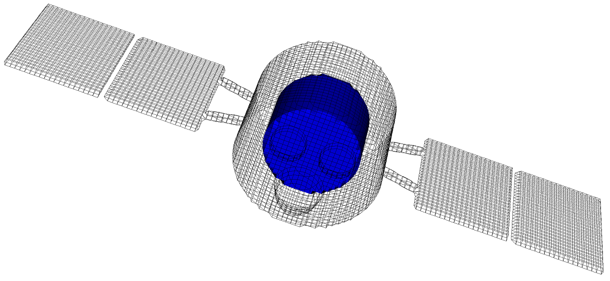
Fig. 625 Visualization of the inner body inside the satellite system.

The phase-space distribution of the positive ions (solarIons species) surrounding the satellite system is shown in Fig. 626 which is obtained after running the simulation for 500 time steps. Solar wind plasma enters into the simulation system from the top z boundary, i.e. above the satellite body.

Fig. 626 Visualization of the satellite system with solar ions.

Surface charge accumulation on the satellite body after 93,000 time steps is shown in Fig. 627. The red dots indicate electrons and the green dots ions. The surface charges on the satellite body can be viewed in VSimComposer by turning on Particle Data –> heavyElectrons and ParticleData -> heavyIons under the Data Overview pane.

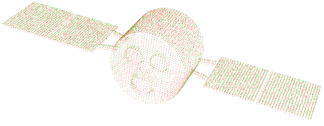
Fig. 627 Visualization of surface charge buildup on the satellite system after 93,000 time steps.

The charge density built-up on the satellite system is shown in Fig. 628 after running for 93,000 time steps. To view the charge density in the simulation domain, turn on the Scalar Data -> rho field in the Data Overview pane. In this figure the satellite body is also included by turning on the Geometries -> poly_surface(Satellite) option in the Data Overview pane. The charge density appears net positive in most regions of the solar panels.

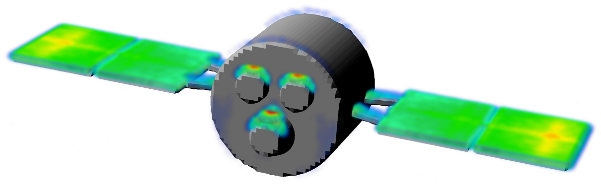
Fig. 628 Visualization of the charge density on the satellite system.

To view the electrostatic potential, turn on phi under the Scalar Data in the Data Overview pane. The electrostatic potential of the satellite system simulated is shown in Fig. 629 after running for 93,000 time steps. The electrostatic potential is plotted in X-Y-Z with domain clipping in the X and Z directions. The bulk of the plasma potential in the space region is close to 0 volts (blue contours). The surface charge built-up on the solar panels raises the surface potential by up to 4 to 5 volts above the bulk space plasma.

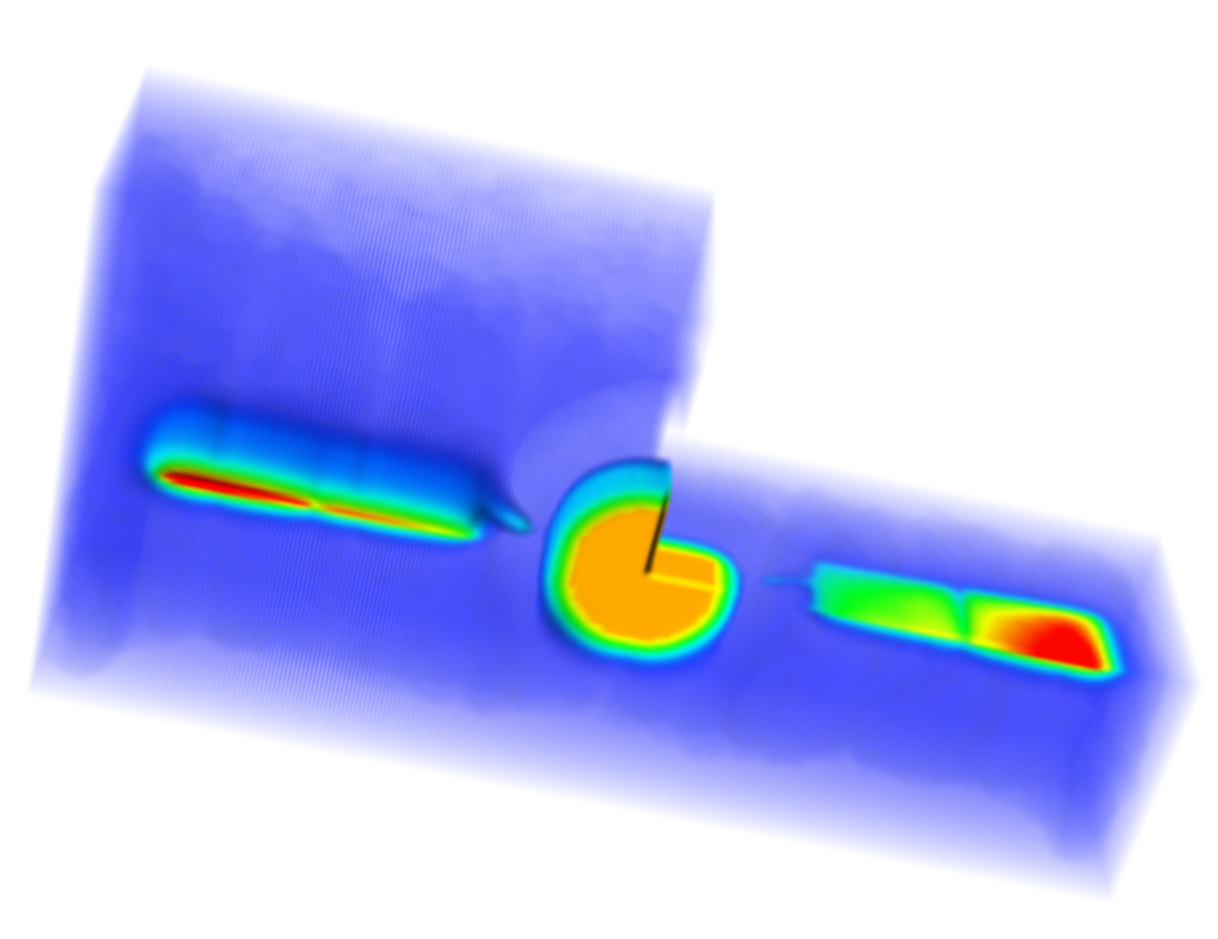
Fig. 629 Visualization of the electric potential surrounding the satellite system.

The magnitude of the electric field distribution on the satellite surface after 93,000 time steps is shown in Fig. 630. The peak of the distribution coincides with regions on the solar array where there is net positive charge buildup. The magnitude of the electric field was computed using the Expressions function in the Visit interface. Should you wish to get to those calculations, right-click on the plot and select Open GUI. (You must have the Enable VisIt context menu box check-marked in Visualization Options. Go to Tools -> Settings -> Visualization Options, to enable this.) This will launch the VisIt control panel. From there, go to Controls -> Expressions. You can select any plottable variable to view its mathematical definition.

Fig. 630 Visualization of the magnitude of electric field surrounding the satellite system.

Further Experiments

The geometry and background space plasma parameters of this input file can be modified to test satellite inner body voltages and satellite surface charge collection in a variety of different space environments.

VSim allows the use of “open” boundary conditions to represent the far-field boundaries in the space environment.