computeEmittanceFromDump.py
This analysis script computes the emittance and associated quantities of a particle beam as it moves through the simulation.
- -s <simname>, --simulationName=<simname>
(string, required)
<simname> is the name of the simulation to be analyzed. The file extension should NOT be included in this text field.
- -S <spname>, --speciesName=<spname>
(string, required)
<spname> is the name of the species to be analyzed.
- -x <N1>, --x1plane=<N1>
(float, optional, default = -1.e6)
If set, excludes particles at x less than this value.
- -X <N2>, --x2plane=<N2>
(float, optional, default = 1.e6)
If set, excludes particles at x greater than this value.
- -n <S>, --numSlices=<S>
(int, optional, default = 1)
This feature allows one to choose the number of slices <S> (between x1plane and x2plane) for the purposes of computing the emittance within each slice.
- -w, --overwrite
(flag)
Whether a dataset or group should be overwritten if it already exists.
Output
This analysis script produces text output specifying the beam parameters it has calculated, and also writes a new history containing the emittance and normalized emittance in x,y (and if 3D, z).
If you are running this analyzer from the GUI, and the output dataset file already exists, then it will be overwritten each time the analyzer is run, unless you uncheck the Overwrite Existing Files box near the bottom of the Analysis Results pane.
If you run the analyzer for multiple slices, and then run it later with a single slice, the datasets for the previous multiple slices are not overwritten, so you will need to delete those datasets first to avoid confusion.
If you are running the analyzer from the command line, the dataset will not be overwritten
unless the -w, or --overwrite flag is specified on the command line.
The results of your analyzer may not be written into the output file if you have not specified the overwrite option to be True.
Usage and Testing
In order to check the output of the analyzer, open the Python file for this analyzer, computeEmittanceFromDump.py (found under your Tech-X Program Files under Contents > engine > bin), and change the verbosity. Find on or around line 25
verbose = 0
and replace it with
verbose = 1
Remember to change this back when you are finished or you will slow down the analyzer.
The following instructions can all be performed from within the VSim Composer GUI. For this example, use the electronBeamDrivenPlasmaT.pre example file, and click on View Input File. Underneath
$ BEAM_GAMMA_INV_2 = BEAM_GAMMA_INV * BEAM_GAMMA_INV
(shortly after 200 lines) insert the text
$ SIGMA_Y_PRIME = 1.e-3
$ SIGMA_Y = BEAM_UX*SIGMA_Y_PRIME
Then in the definition of the velocityGenerator within the species
ElectronBeam (around line 1522), change the expression for
component1.
<STFunc component1>
  kind = expression
  expression = gauss(SIGMA_Y)
</STFunc>
You then have set both \(\sigma_{y}\) and \(\sigma_{y^{\prime}}\), so it is possible to simply calculate the geometric and normalized emittance.
Run this file for 5 steps, dumping every step, and check the box Dump at Time Zero. Then click on the Analyze tab.
Select the computeEmittanceFromDump.py analyzer.
Set up your options as shown using the base name of your input file
(without extension), something like ElectronBeamDrivenPlasma1
and the name of the species for analysis ElectronBeam.
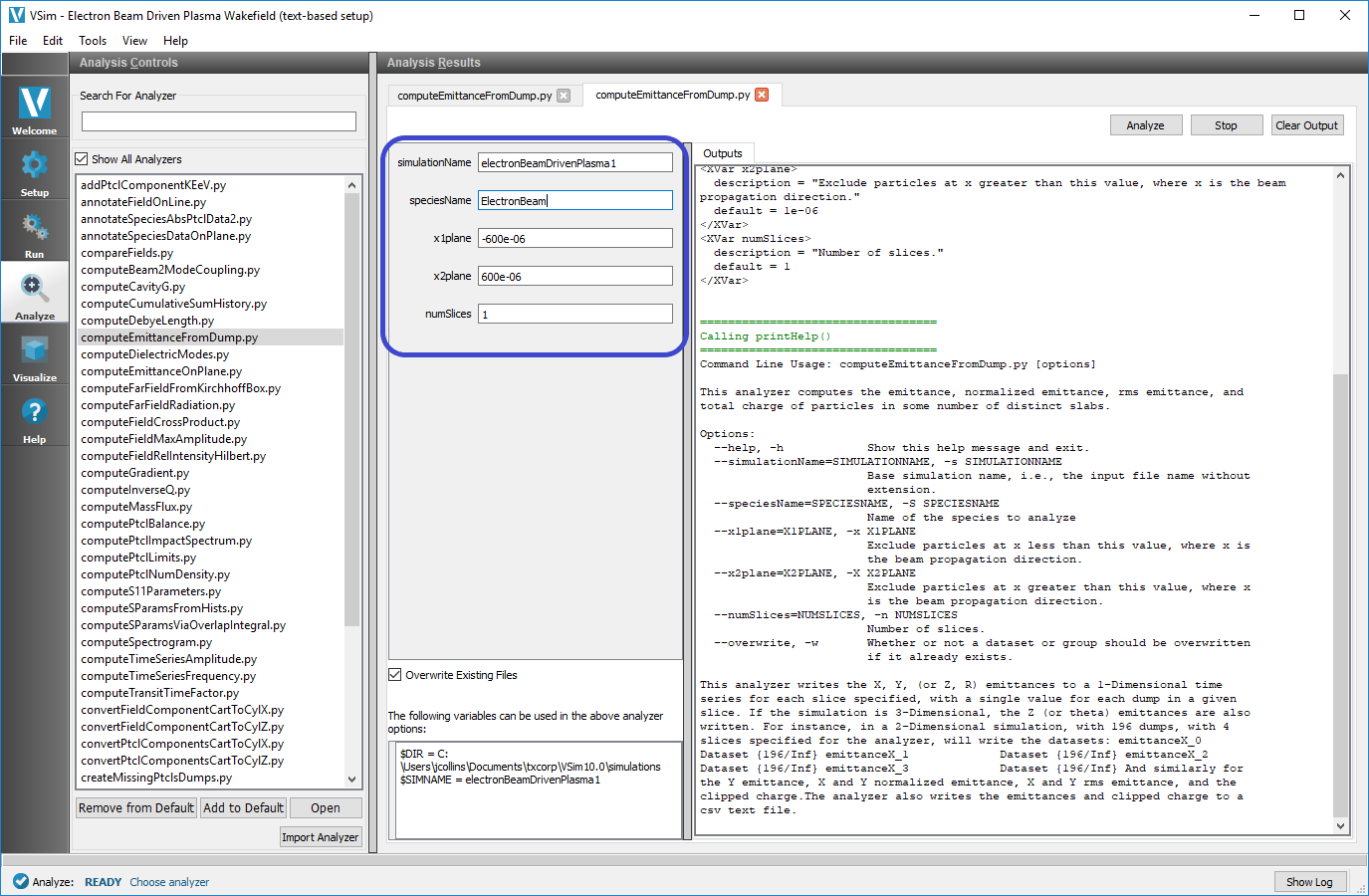
Fig. 629 Setting up the analyzer
Click on Analyze. The output should look something similar to that shown below.
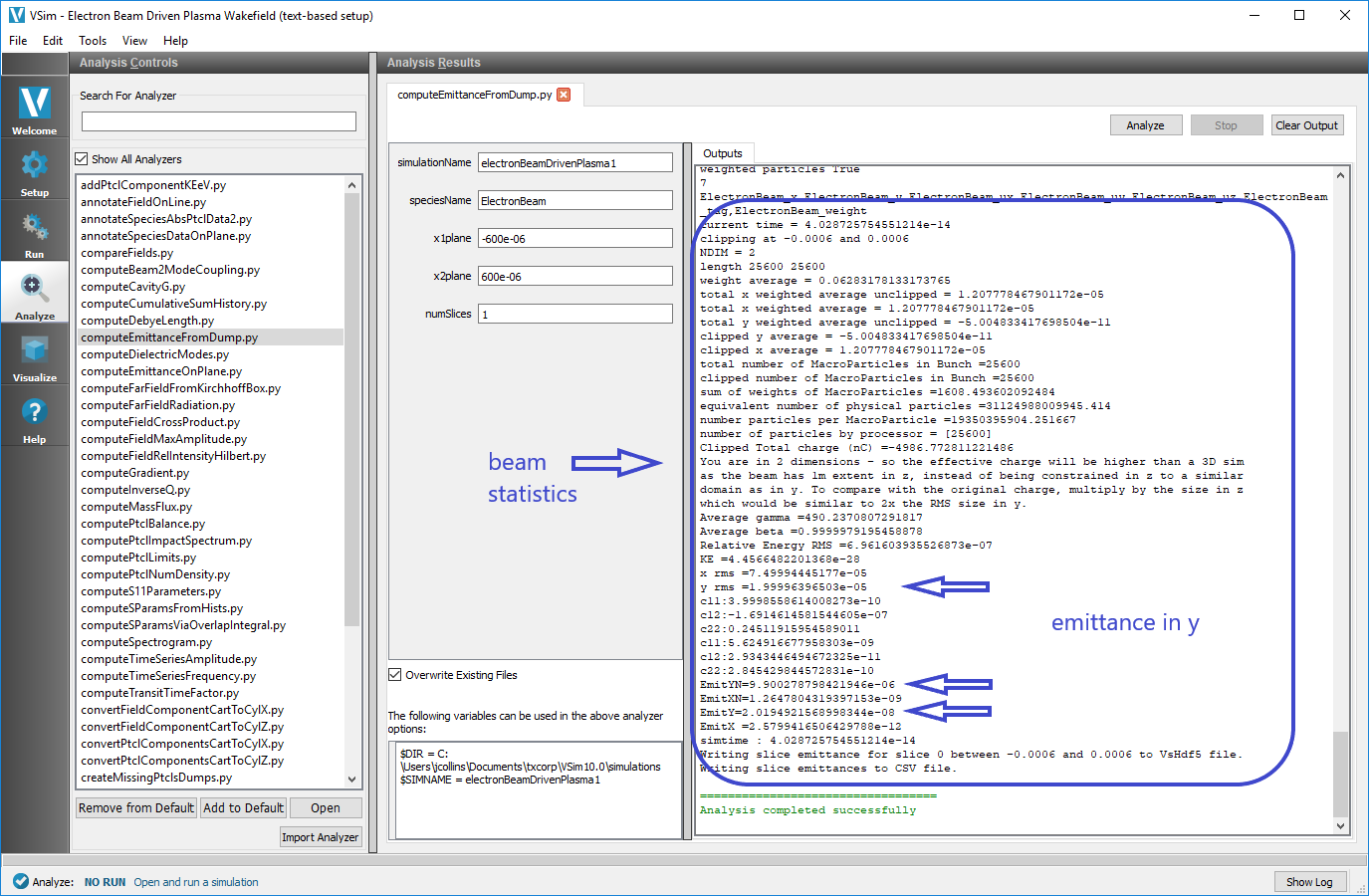
Fig. 630 Analysis output
We can see that our SIGMA_R setting further up the file has translated into \(\sigma_y=2\cdot10^{-5}\), which is shown,
\(\sigma_{y^{\prime}}=1\cdot10^{-3}\), so geometric emittance for this uncorrelated case is \(\epsilon_{y}=2\cdot10^{-8}\).
As \(\gamma=490.2\), the normalized emittance is around under \(\epsilon_{yn}=1\cdot10^{-5}\).
Proceed to the Visualize tab and select the 1-D Fields from the Add a Data View button at top left of the Composer window.
You may want to reload data before looking at the results. This is
demonstrated in Fig. 631. You can see the emittance in y is constant or decreases by a negligible fraction, transferred to the x
component in the self-magnetic field, but due to the beam being completely monoenergetic in x to start, the x emittance grows rapidly.
It is straightforward to add a gaussian function for the BEAM_UX to watch what happens there too.
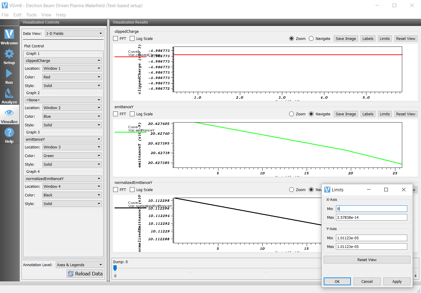
Fig. 631 1-D Fields showing analysis output over time