extractModesViaOperator.py
This analyzer extracts the frequencies and modes of a field from time-series data using the Filter Diagonalization Method (FDM) from [WBC13]. This script is useful for simulations in which one has modes of well defined frequencies, and where only a modest number (<~20) of modes are excited. An example simulation would be that of electromagnetic oscillations rung up by a narrow frequency band of excitation current. The simulation must have been run with uniformly-spaced dumps or with dumps in groups of three for calculation of d / dt or d^2 / dt^2. For example, dumpSteps = [1000 1001 1002 1500 1501 1502 2000 2001 2002 … ] Mode extraction appears to work best when dump groups are spaced at nearly the oscillation period of one of the modes being sought.
- -s <simname>, --simulationName=<simname>
(string, required)
<simname> contains the comma-separated name(s) of the simulation(s) on which modes extraction will be performed.
- -O <outname>, --outputSimName=<outname>
(string, optional)
<outname> is the chosen name for the files output with common data.
- -R <R>, --realFields=<R>
(string, required)
<R> contains the comma-separated name(s) of the real field(s) from which to extract modes. For the d2dt2 operator, fields are treated individually. For the ddt operator, fields are treated as pairs, and so each pair of the list must represent a state vector, e.g., E,B.
- -I <I>, --imagFields=<I>
(string, optional)
<I> contains the comma-separated name(s) of the imaginary field(s) from which to extract modes. For the d2dt2 operator, fields are treated individually. For the ddt operator, fields are treated as pairs, and so each pair of the list must represent a state vector, e.g., EI,BI.
- -F <F>, --secondFieldFactor=<F>
(float, optional)
For ddt operator only, <F> is the factor to multiply second fields by so that they are of comparable magnitude to the first fields.
- -o <op>, --operator=<op>
(string, required, default = ddt)
<op> is one of [d2dt2, ddt]. This is the operator used to extract the modes.
- -d <dr>, --dumpRange=<dr>
(string, required, default = 1 :)
<dr> is the dump range over which to perform mode extraction (in python slice format, but inclusive of the last number).
For example, 1 : 20. If format is e.g. 1 :, the final dump will be detected.
- -S <cs>, --cellSamples=<cs>
(string, required, default = : , : , :)
<cs>, contains the numpy slices for structured field sample selection; for example, 0 , : , : .
- -c <cut>, --cutoff=<cut>
(float, required, default = 1.0e-12)
<cut> is the smallest singular value (relative to largest singular value) to keep.
- -M <M>, --maxNumModes=<M>
(int, optional, default = 0)
<M> is the maximum number of modes to find. -1 means as many as possible.
- -N <N>, --initialModeNumber=<N>
(int, optional, default = 0)
<N> is the index to use for the first mode found.
- -D, --normalizeModes
(int, optional, default = 1)
Normalize modes to the peak value.
- -t, --testing
(int, optional)
Whether using test data or not.
- -w, --overwrite
(flag)
Whether a dataset or group should be overwritten if it already exists.
Output
First, the script prints the singular values of the basis formed
by the midpoint dumps (e.g. dumps 1001, 1501, 2001, … from the
example above). If the singular values of the dump basis fall to
machine precision, mode extraction can be expected to work;
otherwise, more dump groups may be required. Second, the script
prints eigenmode frequencies and wavelengths (c divided by
frequencies), along with extraction errors for each mode found.
Extraction errors indicate how well extracted eigenmodes
approximate a true eigenmode of the chosen operator. Frequencies
are printed to this precision for convenience. Third, if the
construct parameter was set to 1, the script writes eigenmode
fields to vsh5 files that may be viewed in the VSimComposer
Visualize tab. Look for scalar and vector data with names
like E (EigenmodeReal).
If you are running this analyzer from the UI, and the output dataset file already exists, then it will be overwritten each time the analyzer is run, unless you uncheck the Overwrite Existing Files box near the bottom of the Analysis Results pane.
If you are running the analyzer from the command line, the dataset will not be overwritten
unless the -w, or --overwrite flag is specified on the command line.
The results of your analyzer may not be written into the output file if you have not specified the overwrite option to be True.
Usage Recommendations
Current Source
It is recommended that the current source used to excite a cavity take the following form
as depicted in Fig. 635
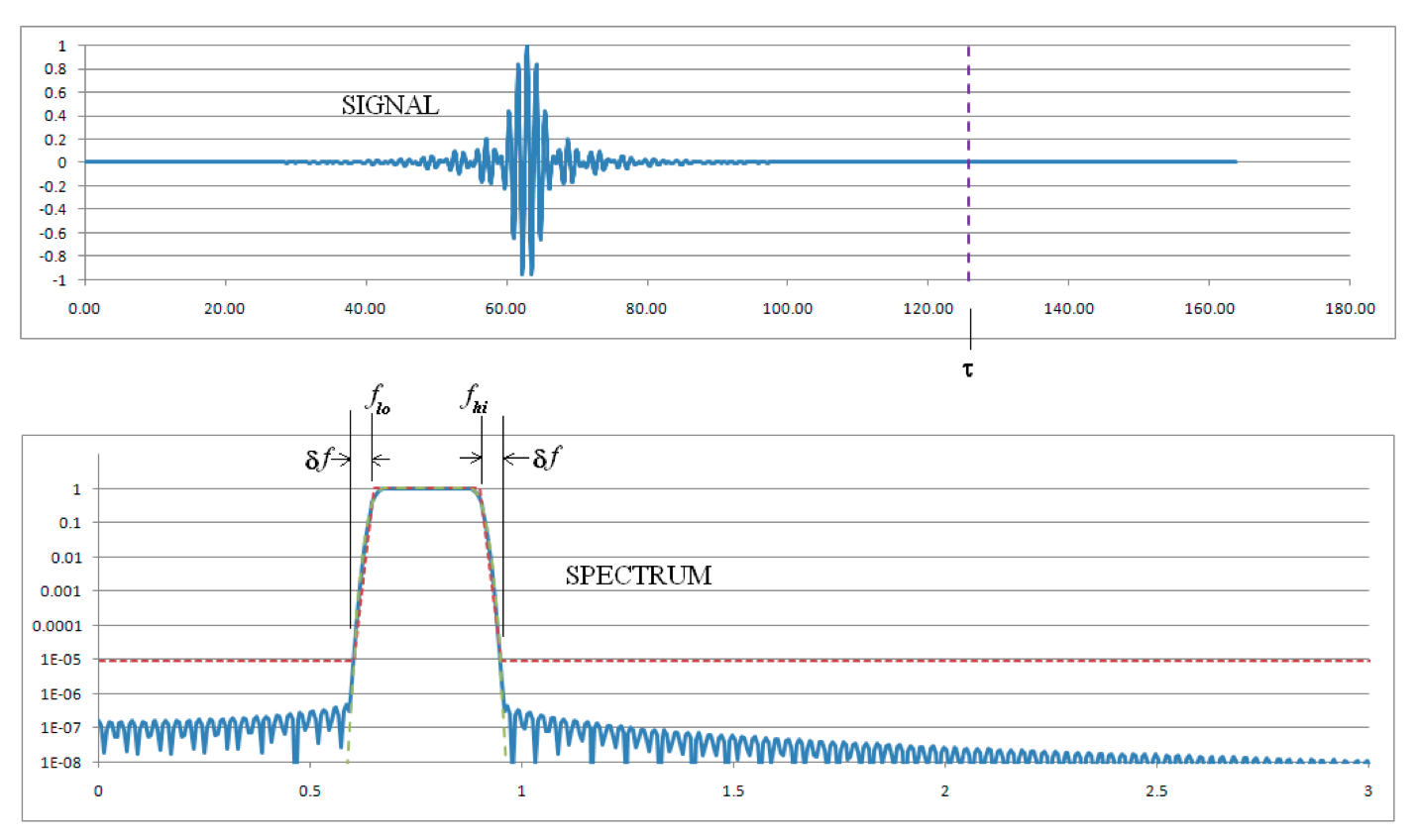
Fig. 635 Time and frequency space plots of current source
\(I_0 = I\left(\tau/2\right)\) is the maximum current, \(\tau = 2 u^2 / \pi \delta f\) is the duration of the excitation, \(f_{lo}\) and \(f_{hi}\) are respectively the lower and upper frequency limits of the excitation, \(H\) is the Heaviside function, and \(\delta f\) and \(u\) together control the steepness of the frequency spectrum near \(f_{lo}\) and \(f_{hi}\). The ratio of the frequency space current source amplitude for frequencies outside the interval \(\left[f_{lo}-\delta f,f_{hi}+\delta f\right]\) to those inside the interval can be specified by the parameter \(u\) with the following table:
Ratio |
\(u\) |
|---|---|
\(10^{-4}\) |
2.76 |
\(10^{-5}\) |
3.13 |
\(10^{-6}\) |
3.46 |
\(10^{-7}\) |
3.77 |
\(10^{-8}\) |
4.06 |
The input parameter initialDump should be set to a dump
for which \(t > \tau\).
Frequency Parameter
There are some rough guidelines for choosing a suitable value of the parameter \(\delta f\):
If examining the low end of a spectrum, where the mode density is not too high, \(\delta f \approx f_{lo} / 4\) is reasonable.
If examining a narrow range of frequencies at the high end of a spectrum, \(\delta f \approx \left(f_{hi}-f_{lo}\right)/4\) is reasonable.
If intentionally trying to exclude modes outside of, but close to, the nominal spectrum from \(f_{lo}\) to \(f_{hi}\), a smaller value of \(\delta f\) may be necessary. If \(\delta f\) is too small, however, heavily damped modes may disappear entirely.
If anticipating modes with loss parameter \(Q_m\) near frequency \(f_m\), \(\delta f\) should satisfy \(\delta f \ge 2 f_m / Q_m\) to ensure the modes are present after the excitation turns off.
For loss-less systems where \(Q \rightarrow \infty\), \(\delta f\) may be as small as desired.
Missing modes may occur if the duration of the simulation is too large, causing modes with finite decay to disappear (in which case, \(\delta f\) should be increased).
Dump Interval and Number
The following are some guidelines for choosing the dump interval
and number of dumps, endingDump - initialDump.
The dump interval should be smaller than half a period of the highest frequency present.
The number of dumps should cover at least one cycle of the smallest frequency present.
There should be at least three times as many dumps as the number of modes found.