External Circuit Model
General Theory
The external circuit module in Vorpal follows the method of V. Vahedi and G. DiPeso [VD97]. In Vorpal this method is extended to three-dimensional electromagnetic and electrostatic solvers, in additional to two-dimensional electrostatics. In principle, the total current, \(J_{t}=\frac{\partial D}{\partial t}+J\), is conserved through the whole system. In the external circuit, the total current \(J_{t}\) is solved from the different equation based on its impedance (resistance R, inductance L, capacitance C) and source components of the circuit. In the simulated plasma region, the total current consists of displacement current \(\frac{\partial D}{\partial t}\) and convective current carried by charged particles \(J\). Matching these two at the boundary provides a time-dependent boundary condition for the simulated plasma region.
Considering a device that is connected to an external circuit via two electrodes, such as a electron gun or plasma discharging chamber, the total electric field between the electrodes is decomposed due to linear superposition as \(\vec{E}_{tot}(t) = \vec{E}(t) + \phi(t)\vec{E}_{0}\), where \(\vec{E}_{tot}(t)\) is the total electric field at time t that is used to advance charged particle dynamics. Electric field \(\vec{E}(t)\) is obtained by solving the Maxwell`s equations for electric (\(\vec{E}\)) and magnetic (\(\vec{B}\)) fields, assuming perfect electric conducting boundary conditions on the two electrodes that are both grounded. \(\phi(t)\) is the time-dependent potential difference between the anode and the cathode that can be measured via pseudopotential. The electric field \(\vec{E}_{0}\) is a constant field that is solved with 1 volt potential difference between the electrodes and no charged particles or currents between them. \(\vec{E}_{0}\) is essentially a vacuum field with unit potential.
The potential \(\phi(t)\) is related to the total charge \(Q(t)\) on one electrode as \(Q(t)=C_{0}\phi(t)\). As there is a fix capacitance \(C_{0}\) for the device when vacuum is assumed, its potential is proportional to the total charge. The charge under 1 volt potential is \(Q_{0}\), thus at any time t, the electrode potential is \(\phi(t)=Q(t)/Q_{0}\). The total field is written as \(\vec{E}_{tot}(t) = \vec{E}(t) + \frac{Q(t)}{Q_{0}}\vec{E}_{0}\), where \(Q(t)\) is calculated at each time step via equations of external circuit, and \(Q_{0}\) can be obtained after solving \(\vec{E}_{0}\).
For a general series RCL circuit as shown in figure Sketch of a plasma simulation with a general RLC external circuit., applying Kirchhoff’s law to the electrode yields the current equation, \(\frac{dQ}{dt} = I_{conv} + I\), where \(I\) is the current in the external circuit that depends on its source and impedance. \(I_{conv}\) is the plasma convection current at the electrode, representing charges emitted or absorbed by the electrode at each time step.
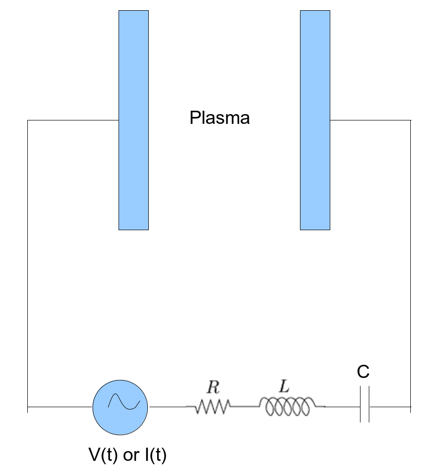
Fig. 625 Sketch of a plasma simulation with a general RLC external circuit.
The voltage equation is obtained by applying Kirchhoff’s law around the circuit, \(L\frac{d^{2}Q_{c}}{dt^{2}}+R\frac{dQ_{c}}{dt}+\frac{Q_{c}}{C} = V(t)-\phi(t)\) where \(Q_{c}\) is the charge in the external circuit capacitor. It is related to the external circuit current via \(I=dQ_{c}/dt\). Substituting this relation into current equation yields \(\frac{dQ}{dt} = I_{conv} + \frac{dQ_{c}}{dt}\). In PIC simulations, the convective current \(I_{conv}\) and the potential difference between two electrodes are defined as \(I_{conv} = I_{emitted} - I_{absorbed}\) and \(\phi(t)=\int\vec{E}(t)dr\). Both can be measured in Vorpal via History blocks. Equations of current and voltage are solved for two unknowns \(Q_{c}(t)\) and \(Q(t)\). Both quantities determine the status of the external circuit and the boundary condition on the electrode.
The voltage equation is solved for capacitor charge \(Q_{c}\) at time step n as \(Q_{c}^{n}=\frac{V(n)-\phi^{n}-K^{n}}{\alpha_{0}}\), where
\(K^{n} = \alpha_{1}Q_{c}^{n-1} + \alpha_{2}Q_{c}^{n-2} + \alpha_{3}Q_{c}^{n-3} + \alpha_{4}Q_{c}^{n-4}\)
\(\alpha_{0} = \frac{9}{4}\frac{L}{\Delta t^{2}} + \frac{3}{2}\frac{R}{\Delta t} + \frac{1}{C}\)
\(\alpha_{1} = -6\frac{L}{\Delta t^{2}} - 2\frac{R}{\Delta t}\)
\(\alpha_{2} = \frac{11}{2}\frac{L}{\Delta t^{2}} + \frac{1}{2}\frac{R}{\Delta t}\)
\(\alpha_{3} = -2\frac{L}{\Delta t^{2}}\)
\(\alpha_{4} = \frac{1}{4}\frac{L}{\Delta t^{2}}\)
The self-consistent solution for charges on the electrode is \(Q^{n} = Q^{n-2} + I_{conv}^{n-1}\cdot 2\Delta t + Q_{c}^{n} - Q_{c}^{n-2}\). Both the potential \(\phi^{n}\) and convective current \(I_{conv}^{n}\) can be measured in Vorpal. Equations of voltage and currents are solved with UserFuncUpdater in Vorpal to obtain the electrode charge \(Q^{n}\) at each time step. \(Q^{n}\) is then coupled with field equation to find the total electric field self-consistently in the system as \(\vec{E}_{tot}(t) = \vec{E}(t) + \frac{Q^{n}}{Q_{0}}\vec{E}_{0}\). Beside the Courant stability condition that is required by the electromagnetic solver, the time step \(\Delta t\) should also follow certain constraints due to external circuits as discussed in reference [VAVB93].
Simulation Procedures
Based on the above algorithm, a simulation with external circuit needs two stage execution. The first stage calculates \(\vec{E}_{0}\) and \(Q_{0}\) that are used in the second stage, where the actual simulation is carried out.
Stage One of the Simulation
The first stage runs a Poisson solver with unit potential in vacuum for only one time step to obtain the electric field \(\vec{E}_{0}\) and the charge on electrode \(Q_{0}\). As the electrodes are represented by GridBoundary, the Poisson solver looks as following
##########
#
# Electrostatic Poisson solver with GridBoundary
#
##########
<EmField myESField>
  kind = yeeStaticEmField

  # set the grid boundary
  gridBoundary = plates

  # Set potential on the grid boundary
  <STFunc boundaryFunc>
      kind = expression
      expression = 1.0*phiFunc(x,y,z)
  </STFunc>

   <Solver mysolver>
      kind = bicgstab
      precond = multigrid
      smoother = GaussSeidel
      nLevels = 7
      tolerance = 1.0e-10
      output = none
      dumpPotential = true
    </Solver>

</EmField>
The total charge on one electrode, such as the cathode used in this example, is calculated with cellFunHist with the following code.
# This is the total charge on the left plate (cathode)
# Its value is important and used for subsequent simulations
# Test its value for convergence
<History totalQ>
  kind = cellFuncHist
  funcLookupScope = myFields
  reduceMethod = sum
  lowerBounds = [0 0 0]
  upperBounds = [$NX/2$ NY NZ]

  <Expression applySteps>
    expression = (mod(n, 1) == 0)
  </Expression>

  <UserFunc histCalc>
    kind = expression

    <CellFunc unitNormal>
      kind = gridBoundaryFunc
      gridBoundary = plates
      result = surfaceOutwardUnitNormal3D
    </CellFunc>

    <CellFunc surfacePos>
      kind = gridBoundaryFunc
      gridBoundary = plates
      result = surfaceCenter
    </CellFunc>

    <CellFunc dArea>
      kind = gridBoundaryFunc
      gridBoundary = plates
      result = surfaceArea
    </CellFunc>

    <SpaceFunc E>
      kind = fieldFunc
      result = fieldValue
      field = myESField.YeeStaticElecFld
      interpolationOrder = 1
      gridBoundary = plates
      polation = fromInOrOutside
      # the following option is not usually recommended
      #boundaryCondition = electricAtPEC
    </SpaceFunc>

    expression = -1.0 * sum(unitNormal(cell) * E(surfacePos(cell))) * EPSILON0 * dArea(cell)
  </UserFunc>

  resultVecDescriptions = ["sum of total charge"]
  # following is a rough memory size (in MB) that can always be
  # obtained: it's (very) small here for testing; normally it's best to
  # use the default value.
  maxMemChunkSize = 9.6e-5 # about 100 B
  # to use such a small value for testing, we need to set the following
  allowSmallMaxMemChunkSize = true
  checkForUnaccessedAttribs = 2
</History>
After the run of this first stage, totalQ (\(Q_{0}\)) is read from the hdf5 file for History. It values, together with the electrostatic field (YeeStaticElecFldTrilinos), are used for stage two.
Stage Two of the Simulation
Stage two is to run the actual simulation that is coupled with external circuit. The convective current at the cathode is measured with the following two History blocks for emitted and absorbed currents.
<History cathodeEmitCurrent>
  kind = speciesCurrEmit
  species = [electrons]
  ptclEmitter = electrons.psource
</History>

<History cathodeAbsCurrent>
  kind = speciesCurrAbs
  species = [electrons]
  ptclAbsorbers = [cathodeAbs]
</History>
The electrostatic field at unit potential calculated from stage one is imported to an edge field name unitE0. It is imported from hdf5 file and only needs to update once at the beginning of the simulation.
<FieldUpdater initunitE0Updater>
  kind = importFromFileUpdater
  fileName = "./externalCircuit0_YeeStaticElecFldTrilinos_1.h5"
  dataset = "YeeStaticElecFldTrilinos"
  writeFields = [unitE0]
  writeComponents = [0 1 2]
  lowerBounds = [0   0   0]
  upperBounds = [NX1 NY1 NZ1]
</FieldUpdater>
Charges on the capacitor of external circuit and one of the electrodes are updated via two updaters that solve external circuit voltage and current equations. Q0 used in the chargeQUpdater is obtained form stage one simulation.
# This updated the Q at the capacitor C at time step n
# according to the external circuit voltage equation (Kirchoff's voltage law)
# Here the cuircuit is assumed to a general series RLC
<FieldUpdater capacitorQUpdater>
  kind = userFuncUpdater
  lowerBounds = [0 0 0]
  upperBounds = [NX1 NY1 NZ1]

  readFields = [phiField capacitorQnm1 capacitorQnm2 capacitorQnm3 capacitorQnm4]
  readComponents = [0 0 0 0 0]
  readFieldVarNames = [phi qnm1 qnm2 qnm3 qnm4]

  writeFields = [capacitorQn]
  writeComponents = [0]
  maxNumEvals = 64

  <UserFunc updateFunction>
    kind = expression
    $alpha0 = 2.25*L/DT/DT + 1.5*R/DT + 1/C
    $alpha1 = -6.0*L/DT/DT - 2.0*R/DT
    $alpha2 = 5.5*L/DT/DT + 0.5*R/DT
    $alpha3 = -2.0*L/DT/DT
    $alpha4 = 0.25*L/DT/DT
    expression = (Vsource((n)*dt) - phi - alpha1*qnm1 - alpha2*qnm2 - alpha3*qnm3 - alpha4*qnm4) / alpha0
  </UserFunc>
</FieldUpdater>


<FieldUpdater chargeQUpdater>
  kind = userFuncUpdater
  lowerBounds = [0 0 0]
  upperBounds = [NX1 NY1 NZ1]

  readFields = [totalQnm2 capacitorQn capacitorQnm2]
  readComponents = [0 0 0]
  readFieldVarNames = [qnm2 qcn qcnm2]

  writeFields = [totalQn]
  writeComponents = [0]
  maxNumEvals = 64

  <UserFunc updateFunction>
    kind = expression
    expression = qnm2 + (qcn - qcnm2) - 2.0*dt*(emitI - absI)
  </UserFunc>
</FieldUpdater>
Assuming both electrodes are perfect electric conductors, edgeE and faceB are solved with regular Faraday, Ampere and Dey-Mittra updaters. Combining edgeE with scaled unitE, we obtain the totalE field that is use to advance charged particles dynamics via Lorenz force together with faceB.
<FieldUpdater totalEUpdater>
  kind = userFuncUpdater
  lowerBounds = [0 0 0]
  upperBounds = [NX1 NY1 NZ1]

  readFields = [edgeE edgeE edgeE unitE0 unitE0 unitE0 totalQn]
  readComponents = [0 1 2 0 1 2 0]
  readFieldVarNames = [EX EY EZ E0X E0Y E0Z QN]

  writeFields = [totalE totalE totalE]
  writeComponents = [0 1 2]
  maxNumEvals = 64

  <UserFunc updateFunction>
    kind = expression
    expression = tensorProd(EX, EY, EZ) + tensorProd(E0X, E0Y, E0Z) * QN / Q0
  </UserFunc>
</FieldUpdater>
Notes for External Circuit
UserFuncs are heavily used in the external circuit module. Users are suggested to read relevant sections about UserFuncs. In the capacitorQUpdater, phi is measured via pseudopotential and read into a field via historySTFunc. For their usage, please refer to the sections about feedback and historySTFunc in VSim Reference.